Week 8: Literature review - RANS derivation and analysis

AIM : 

Apply reynold's decomposition to the NS equations and come up with the expression for reynold's stress.

• Explain your understanding of the terms reynold's stress
• What is turbulent viscosity? How is it different from molecular viscosity?

RANS MODELLING:

The RANS approach decomposes flow variables (e.g. velocity) into mean and fluctuating terms.

       ui=u¯i+ui′">ui=¯ui+ui'

i.e, instantaneous velocity= mean velocity(we are solving for) + fluctuating velocity( we are going for modelling).

                 

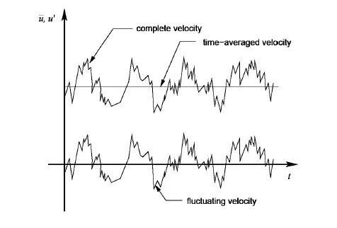
 Now, inserting the above equation into the NS equation and averaging the result yields the RANS equation.

Governing equation for the boundary layer:

∂u∂x+∂v∂y=0">∂u∂x+∂v∂y=0

        continuity equation

 ρ(∂u∂t+u∂u∂x+v∂u∂y)=-∂p∂x+μ(∂2u∂y2+∂2u∂x2)">ρ(∂u∂t+u∂u∂x+v∂u∂y)=−∂p∂x+μ(∂2u∂y2+∂2u∂x2)

        momentum equation

  If we take origina; N.S equation and solve it over small time scale and if we have large number of computational cell, then

we do not need turbulence model.

So, wit the help of turbulence model we can capture the effect of turbulence with coarser grid and larger time step.

Hence,we are taking the governing equation and integrating over a time that is much larger than turbulent time scale ,this is

called averaging.

now , Reynolds decomposition follows:

                     u(x,y,z,t)=u¯(x,y,z)+u′(x,y,z,t)">u(x,y,z,t)=¯u(x,y,z)+u'(x,y,z,t)

similarly for V and W velocity components.

 lets apply decomposition to continuity equation:

  ∂∂x(u¯+u′)+∂∂y(v¯+v′)=0">∂∂x(¯u+u')+∂∂y(¯v+v')=0

 1ti∫0ti(∂∂x(u¯+u′)dt+1ti∫0ti∂∂y(v¯+v′)dt=0">1ti∫ti0(∂∂x(¯u+u')dt+1ti∫ti0∂∂y(¯v+v')dt=0

 1ti∫∂∂xu¯dt+1ti∫∂∂xu′dt+1ti∫∂∂yv¯dt+1ti∫∂∂yv′dt=0">1ti∫∂∂x¯udt+1ti∫∂∂xu'dt+1ti∫∂∂y¯vdt+1ti∫∂∂yv'dt=0

 1ti∫∂∂xu¯dt+1ti∫∂∂yv¯dt=0">1ti∫∂∂x¯udt+1ti∫∂∂y¯vdt=0

∂∂xu¯⋅(1ti)∫0tidt+∂∂yv¯⋅(1ti)∫0tidt=0">∂∂x¯u⋅(1ti)∫ti0dt+∂∂y¯v⋅(1ti)∫ti0dt=0

∂∂xu¯(ti-0ti)+∂∂yv¯(ti-0ti)=0">∂∂x¯u(ti−0ti)+∂∂y¯v(ti−0ti)=0

∂∂xu¯+∂∂yv¯=0">∂∂x¯u+∂∂y¯v=0

  time averaging velocity component satisfies the continuity equation.

 Now momentum equation:

ρ{∂u∂t+u⋅∂u∂x+v⋅∂u∂y}=-∂P∂x+μ⋅∂2u∂y2">ρ{∂u∂t+u⋅∂u∂x+v⋅∂u∂y}=−∂P∂x+μ⋅∂2u∂y2

∂u∂t+u⋅∂u∂x+v⋅∂u∂y=-∂p∂x+(μρ)⋅(∂2u∂y2)">∂u∂t+u⋅∂u∂x+v⋅∂u∂y=−∂p∂x+(μρ)⋅(∂2u∂y2)

∂u∂t+u⋅∂u∂x+v⋅∂u∂y+u(∂u∂x+∂v∂y)=(1ρ)-∂P∂x+ν∂2u∂y2">∂u∂t+u⋅∂u∂x+v⋅∂u∂y+u(∂u∂x+∂v∂y)=(1ρ)−∂P∂x+ν∂2u∂y2

                              In this equation x component of velocity is multiplied by continuity equation.

Now rearranging the terms we get,

 ∂u∂t+u⋅∂u∂x+v⋅∂u∂y+u⋅∂u∂x+u⋅∂v∂y=-(1ρ)∂P∂x+ν⋅∂2u∂y2">∂u∂t+u⋅∂u∂x+v⋅∂u∂y+u⋅∂u∂x+u⋅∂v∂y=−(1ρ)∂P∂x+ν⋅∂2u∂y2

∂u∂t+(∂u2∂x)+∂∂y(u⋅v)=-(1ρ)⋅∂p∂x+ν∂2u∂y2">∂u∂t+(∂u2∂x)+∂∂y(u⋅v)=−(1ρ)⋅∂p∂x+ν∂2u∂y2

 Now Reynolds decomposition follows:

u=u¯+u′">u=¯u+u'

 1ti⋅∫0ti(∂∂t(u¯+u′)dt)+∂∂y(u¯+u′)(v¯+v′)dt+∂∂x(u¯+u′)2dt=1ti∫0ti{-∂ρ∂x(P¯+P′)dt}+ν∂2∂y2(u¯+u′)dt">1ti⋅∫ti0(∂∂t(¯u+u')dt)+∂∂y(¯u+u')(¯v+v')dt+∂∂x(¯u+u')2dt=1ti∫ti0{−∂ρ∂x(¯¯¯P+P')dt}+ν∂2∂y2(¯u+u')dt

 1ti(∫0ti∂u¯∂tdt+∂u′∂tdt+∂u¯2∂xdt+∂u′2∂xdt+(∂(2⋅u¯⋅u′∂x)dt+∂∂y(u¯v¯)dt+∂∂y(u¯v′)dt+∂∂y(u′v¯)dt+∂∂y(u′v′)dt=1ti∫0ti(-1ρ⋅∂P¯∂xdt-(1ρ)⋅∂P′∂xdt">1ti(∫ti0∂¯u∂tdt+∂u'∂tdt+∂¯u2∂xdt+∂u'2∂xdt+(∂(2⋅¯u⋅u'∂x)dt+∂∂y(¯u¯v)dt+∂∂y(¯uv')dt+∂∂y(u'¯v)dt+∂∂y(u'v')dt=1ti∫ti0(−1ρ⋅∂¯¯¯P∂xdt−(1ρ)⋅∂P'∂xdt

+ν∂2u¯∂y2dt+ν∂2u′∂y2dt">ν∂2¯u∂y2dt+ν∂2u'∂y2dt

∂u¯∂t+∂u¯2∂x+∂∂y(u¯⋅v¯)=-(1ρ)⋅∂P¯∂x+ν⋅∂2u¯∂y2-(1ti)∫0ti∂∂x(u′2dt)-(1ti)∫0ti∂∂y(u′v′)dt">∂¯u∂t+∂¯u2∂x+∂∂y(¯u⋅¯v)=−(1ρ)⋅∂¯¯¯P∂x+ν⋅∂2¯u∂y2−(1ti)∫ti0∂∂x(u'2dt)−(1ti)∫ti0∂∂y(u'v')dt

since the velocity gradient in'x' direction is lower as compared to 'y' direction so, 1ti∫0ti∂∂x(u′)2dt">1ti∫ti0∂∂x(u')2dt

tends to zero.

Therfore, ∂u¯∂t+∂u¯2∂x+∂u¯v¯∂y=-1ρ∂P¯∂x+ν⋅∂2u¯∂y2-(1ti)∫0ti∂(u′v′)∂ydt">∂¯u∂t+∂¯u2∂x+∂¯u¯v∂y=−1ρ∂¯¯¯P∂x+ν⋅∂2¯u∂y2−(1ti)∫ti0∂(u'v')∂ydt

  = -(1ρ)⋅∂P¯∂x+(1ρ)∂∂y[ν⋅∂u¯∂y-ρti∫0t-i(u′v′)dt]">−(1ρ)⋅∂¯¯¯P∂x+(1ρ)∂∂y[ν⋅∂¯u∂y−ρti∫t−i0(u'v')dt]

  The left hand side denotes the inertial term calculated based on average quantity.

The right hand side denotes momentum diffusion i.e, combination of molecular viscosity(first term) and turbulent

viscosity(2nd term).

Turbulance modelling is all about capturing the time integral of (u'v')dt i.e, Reynolds stress.

In the viscous sub-layer the viscous term is much much greater than the inertial term and assuming insignificant pressure

drop, dp/dx->0

we have the equation : -1ρ⋅∂P¯∂x+(1ρ)∂∂y[ν⋅∂u¯∂y-ρti∫0ti(u′v′)dt]">−1ρ⋅∂¯¯¯P∂x+(1ρ)∂∂y[ν⋅∂¯u∂y−ρti∫ti0(u'v')dt]

                                            μ⋅∂u¯∂y-ρti∫0ti(u′v′)dt=const.">μ⋅∂¯u∂y−ρti∫ti0(u'v')dt=const.

inside viscous sub-layer molecular viscosity dominates When we are in outside the viscous sub-layer, generally turbulent viscosity dominates. so Reynolds stress is τs">τs equal to

 τs=-ρti∫0ti(u′v′)dt">τs=−ρti∫ti0(u'v')dt

approx

 Generally the turbulent transfer of momentum by eddies giving rise to an internal fluid friction but taking place inmuch

larger scale.

 Wheras the molecular viscosity is the transfer of momentum (motion) by random motions of individual molecules not moving

together.

Eddy Viscosity Versus Molecular Viscosity

Joseph Valentin Boussinesq was the first to attack the closure problem, by introducing the concept of eddy viscosity. In 1877 Boussinesq proposed relating the turbulence stresses to the mean flow to close the system of equations. Here the Boussinesq hypothesis is applied to model the Reynolds stress term. Note that a new proportionality constant  0" aria-hidden="true" />, the turbulence eddy viscosity, has been introduced. Models of this type are known as eddy viscosity models or EVM's.

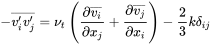
Which can be written in shorthand as

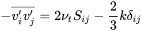
where  is the mean rate of strain tensor

           is the turbulence eddy viscosity

 is the turbulence kinetic energy

and  is the Kronecker delta.

In this model, the additional turbulence stresses are given by augmenting the molecular viscosity with an eddy viscosity. This can be a simple constant eddy viscosity (which works well for some free shear flows such as axisymmetric jets, 2-D jets, and mixing layers).

At a molecular level, viscosity is a result the interaction between the different molecules in a fluid. This can be also understood as friction between the molecules in the fluid. Just like in the case of friction between moving solids, viscosity will determine the energy required to make a fluid flow.  

CONCLUSION

1. The RANS derivation and analysis was conduced
2. Turbulence model of RANS was interpreted