Backward Facing step using multiple meshes refining mesh grading factors inside BlockMeshDict file of BlockMesh using OpenFOAM.
OBJECTIVE:
To create a geometry and simulate a 2D flow through a Backward Facing step using multiple meshes refining mesh grading factors inside BlockMeshDict file of BlockMesh using OpenFOAM.
Problem Statement:
Mesh specification
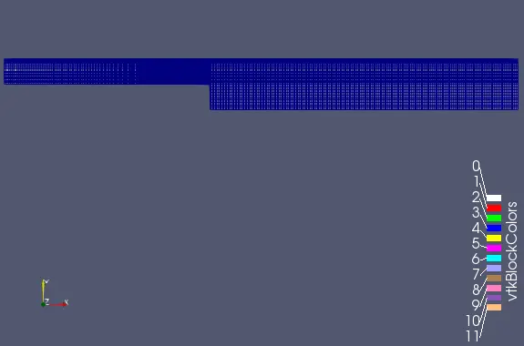
- Number of cells along the x direction (longer dimension) = 200
- Number of cells along the y direction = 10
- Use a graded mesh. Grading factor near all walls should be 0.2
THEORY:
Computational Fluid Dynamics (CFD) is the branch of CAE that simulates fluid motion and heat transfer using numerical approaches. The software we use here to simulate the flow is OpenFoam.
OpenFOAM (Open-source Field Operation And Manipulation) is a C++ toolbox for the development of customized numerical solvers, and pre-/post-processing utilities for the solution of continum mechanics problems, most prominently including Computational Fluid Dynamics(CFD).
Boudary Layer- It is the locus of the point at which the velocity of the fluid becomes equal to 99% of the freestream velocity. It is the region in the flow field inside which a fulid flows with high relative velocity. It is the region beyond which there exist no relative motion. The thickness of the boundary layer is the function of direction of flow. As the fluid flow propogates the nature of the Boundary layer also changes as per the type of flow depending wheather it is laminar, transient and turbulent.
Boundary layer separation:
It is nothing but the detachment of boundary layer from a surface. The fluid exerts a constant pressure on the surface once it has separated instead of a continually increasing pressure if still attached. Separation of the boundary layers occurs whenever the flow tries to decelerate quickly, that is whenever the outer pressure gradient is negative, or the pressure gradient is positive, sometimes referred to as an adverse pressure gradient
Flow separation occurs when the velocity at the wall is zero or negative and an inflection point exists in the velocity profile and a positive or adverse pressure gradient occurs in the direction of flow.
In fluid Dynamics, the no-slip condition for viscous fluids assumes that at a solid boundary, the fluid will have zero velocity relative to the boundary.The fluid velocity at all fluid–solid boundaries is equal to that of the solid boundary.
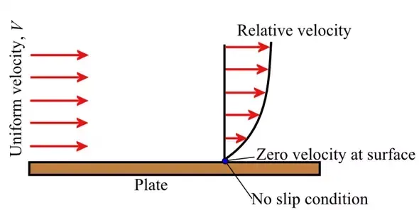
Operating System and Interface
Operating System used here is Linux - Ubuntu. Hence OpenFoam is a Command Line Interface (CLI), it uses text-based user interface (UI) used to view and manage computer files.
Commands Used:
tut - tutorial
app - applications
sol - solver
cp - copy
rm - remove
ls - list
gedit - used to open text editors
./ - Run
cd - Change directory
cd .. - Change to previous directory
mkdir - Make Directory
$FOAM_RUN - navigates to OpenFoam run directory
paraFoam - opens paraview where the simulation is represented
EXPLANATION:
Steps to be done
- Choosing a Solver
- Creating Geometry
- Editing BlockMeshDict file
A) Boundary Conditions
B) Intial Conditions
1) Pressure
2) Velocity - Editing ControlDict file
- Comparision of various Grading schemes
Velocity Profile & Line Plot - Conclusion
Detail Explanation:
- The 'tutorial' folder in OpenFoam folder is opened and the 'incompressible' directory is opened.
- Then the 'cavity' is selected and opened, inside of which there exists another 'cavity' folder.
- This 'cavity' folder is copied into 'run' folder and renamed as 'Drill_down'
- Later on we navigate into 'solver' folder, inside of which there exists an 'incompressible' directory (similar to that in 'tutuorials')
- There is a solver called 'icoFoam' inside the 'incompressible'. This is the solver we are supposed to use for this simulation.
- Now we go to the 'run' folder, and open the 'Drill_down' directory.
- There will be 'p' and 'U' inside 'Drill_down'. The 'p' directory stands for pressure and it needs to be edited in gedit as per our requirements. The 'U' directory stands for Velocity and it also needs to be edited in gedit as per our requirements.
- Next the System directory is selected from directory 'Drill_down', inside of which there exists 'blockMeshDict' , 'controlDict', 'fvSchemes', 'fvSolutions'.
- The 'fvSchemes' and 'fvSolutions' are methods and need not be edited
- The 'blockMeshDict' has to be edited according to our part design which we have prepared and structured earlier in paper.
- The 'controlDict' also has to be edited according to our part design which we have prepared and structured earlier in paper.
- Next, we type in 'blockMesh' command to initiate the mesh.
- Then the solver which we have reffered to earlier is typed in as 'icoFoam'. The result is obtained. To get a graphical view type in 'paraFoam'.
- Do this for the grading factors 0.2, 0.5, 0.8.
- Then we compare velocity magnitude contours near the step region for the mesh grading factor of 0.2, 0.5, 0.8.
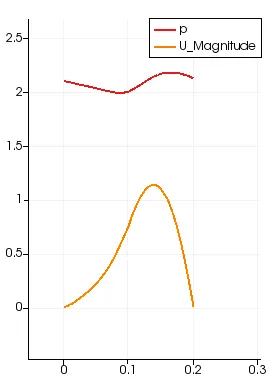
- Measure the velocity profile at 0.085 m from the inlet of the geometry.
Solver:
Since we need a solver which solves a Incompressible Laminar Navier Stokes Equation (Continuity and Momentum), we choose icoFoam which is present as an inbuilt directory in OpenFoam software.
Inside icoFoam solver, cavity is selected for the project.
Creating Geometry
The below SolidWorks figure represents the geometry to be created by using BlockMeshDict file (present in tutorial/systems) with the same specifications shown below
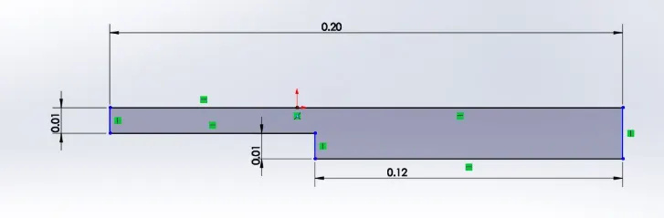
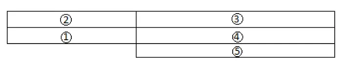
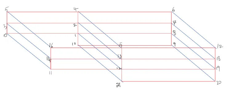
The BlockMeshDict file is modified to create geometry using Backward Facing Step. Hence it can only be done in blocks, we have considered it as 5 different blocks(1st pic) and the indexed the vertices(2nd pic) inas shown below.
1)Distribution of Blocks
2)Indexing the Vertices
BlockMeshDict file
/*--------------------------------*- C++ -*----------------------------------*
  =========                 |
        /  F ield         | OpenFOAM: The Open Source CFD Toolbox
       /   O peration     | Website:  https://openfoam.org
      /    A nd           | Version:  8
     /     M anipulation  |
*---------------------------------------------------------------------------*/
FoamFile
{
    version     2.0;
    format      ascii;
    class       dictionary;
    object      blockMeshDict;
}
// * * * * * * * * * * * * * * * * * * * * * * * * * * * * * * * * * * * * * //

convertToMeters 1;

vertices
(
    (0 0 0)		//vertex no.0
    (0.08 0 0)		//vertex no.1
    (0.08 0.005 0)	//vertex no.2
    (0 0.005 0)	//vertex no.3
    (0.08 0.01 0)	//vertex no.4
    (0 0.01 0)		//vertex no.5
    (0.2 0.01 0)	//vertex no.6
    (0.2 0.005 0)	//vertex no.7
    (0.2 0 0)		//vertex no.8
    (0.2 -0.01 0)	//vertex no.9
    (0.08 -0.01 0)	//vertex no.10
    (0 0 0.001)	//vertex no.11
    (0.08 0 0.001)	//vertex no.12
    (0.08 0.005 0.001)	//vertex no.13
    (0 0.005 0.001)	//vertex no.14
    (0.08 0.01 0.001)	//vertex no.15
    (0 0.01 0.001)	//vertex no.16
    (0.2 0.01 0.001)	//vertex no.17
    (0.2 0.005 0.001)	//vertex no.18
    (0.2 0 0.001)	//vertex no.19
    (0.2 -0.01 0.001)	//vertex no.20
    (0.08 -0.01 0.001)	//vertex no.21

);

blocks
(
    //CODE SPLIT UP
    //Vertex no. hex()
    //no. of cells in (x y z)
    //streching of cells simpleGrading (x y z)

    hex (0 1 2 3 11 12 13 14) (200 10 1) simpleGrading (1 1 1)
    hex (3 2 4 5 14 13 15 16) (200 10 1) simpleGrading (1 1 1)
    hex (2 7 6 4 13 18 17 15) (200 10 1) simpleGrading (1 1 1)
    hex (1 8 7 2 12 19 18 13) (200 10 1) simpleGrading (1 1 1)
    hex (10 9 8 1 21 20 19 12) (200 10 1) simpleGrading (1 1 1)
);

edges
(
);

boundary
(
    inlet
    {
        type patch;
        faces
        (
            (0 11 14 3)
            (3 14 16 5)
        );
    }

    outlet
    {
        type patch;
        faces
        (
            (20 9 8 19)
            (19 8 7 18)
            (18 7 6 17)
        );
    }

    front
    {
        type empty;
        faces
        (
            (11 12 13 14)
            (14 13 15 16)
            (13 18 17 15)
            (12 19 18 13)
            (21 20 19 12)
        );
    }

    Back
    {
        type empty;
        faces
        (
            (3 2 1 0)
            (5 4 2 3)
            (4 6 7 2)
            (2 7 8 1)
            (1 8 9 10)
        );
    }

    Bottom
    {
        type wall;
        faces
        (
            (0 1 12 11)
            (10 9 20 21)
        );
    }

    Top
    {
        type wall;
        faces
        (
            (4 5 16 15)
            (6 4 15 17)
        );
    }

    Stepside
    {
        type wall;
        faces
        (
            (1 10 21 12)
        );
    }
);

mergePatchPairs
(
);

// ************************************************************************* //
Boundary Conditions
After defining the boundaries correctly, to check if you have given defined them correctly, execute the blockMesh command in the terminal.Now open paraFoam, select all the patches and click apply. You will now be able to see the boundary conditions that have been applied to the geometry.
2. controlDict file.
This text file is used to edit the values of time steps along initial and final time.
/*--------------------------------*- C++ -*----------------------------------*
  =========                 |
        /  F ield         | OpenFOAM: The Open Source CFD Toolbox
       /   O peration     | Website:  https://openfoam.org
      /    A nd           | Version:  7
     /     M anipulation  |
*---------------------------------------------------------------------------*/
FoamFile
{
    version     2.0;
    format      ascii;
    class       dictionary;
    location    "system";
    object      controlDict;
}
// * * * * * * * * * * * * * * * * * * * * * * * * * * * * * * * * * * * * * //

application     icoFoam;

startFrom       startTime;

startTime       0;

stopAt          endTime;

endTime         0.05;

deltaT          0.0005;

writeControl    timeStep;

writeInterval   20;

purgeWrite      0;

writeFormat     ascii;

writePrecision  6;

writeCompression off;

timeFormat      general;

timePrecision   6;

runTimeModifiable true;


// ************************************************************************* //
3. Velocity code.
/*--------------------------------*- C++ -*----------------------------------*
  =========                 |
        /  F ield         | OpenFOAM: The Open Source CFD Toolbox
       /   O peration     | Website:  https://openfoam.org
      /    A nd           | Version:  7
     /     M anipulation  |
*---------------------------------------------------------------------------*/
FoamFile
{
    version     2.0;
    format      ascii;
    class       volVectorField;
    object      U;
}
// * * * * * * * * * * * * * * * * * * * * * * * * * * * * * * * * * * * * * //

dimensions      [0 1 -1 0 0 0 0];

internalField   uniform (0 0 0);

boundaryField
{
    Inlet
      {
        type            fixedValue;
        value           uniform (1 0 0);
      }

     Outlet
      {
        type            zeroGradient;
      }

    top_and_bottom
     {
        type            noSlip;
     }

    frontAndBack
     {
        type            empty;
     }
}

// ************************************************************************* //
4. Preassure code.
/*--------------------------------*- C++ -*----------------------------------*
  =========                 |
        /  F ield         | OpenFOAM: The Open Source CFD Toolbox
       /   O peration     | Website:  https://openfoam.org
      /    A nd           | Version:  7
     /     M anipulation  |
*---------------------------------------------------------------------------*/
FoamFile
{
    version     2.0;
    format      ascii;
    class       volScalarField;
    object      p;
}
// * * * * * * * * * * * * * * * * * * * * * * * * * * * * * * * * * * * * * //

dimensions      [0 2 -2 0 0 0 0];

internalField   uniform 0;

boundaryField
{
    Inlet
    {
        type            zeroGradient;
    }

    Outlet
    {
        type            fixedValue;
        value           uniform 0;
    }

    frontAndBack
    {
        type            empty;
    }

    top_and_bottom
    {
        type           zeroGradient;
    }
}

// ************************************************************************* //Results:-
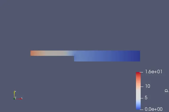
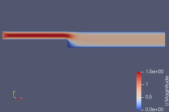
1.When mesh grading factor is taken to be 0.2 along the walls.

a. Mesh Profile.
b. Preassure Profile.
c.Velocity profile.
d. Variation Velocity and Preassure profile at 0.085 m from the inlet of geometry for grading = 0.2.
length of Y-axis
2.When mesh grading factor is taken to be 0.5 along the walls.

a. Mesh Profile.
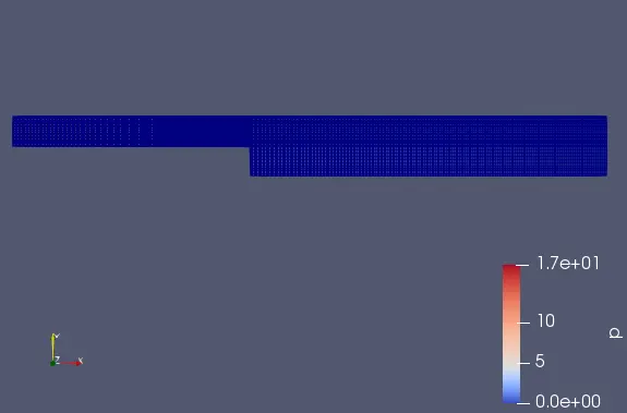
b. Preassure profile.
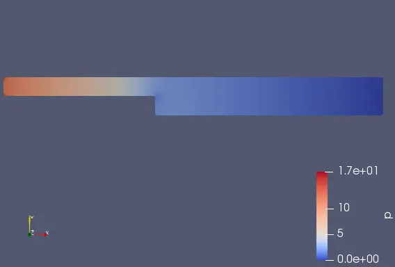
c. Velocity profile.
d. Variation Velocity and Preassure profile at 0.085 m from the inlet of geometry for grading = 0.2.
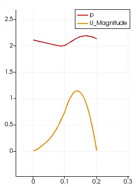
length of Y-axis
3. When mesh grading factor is taken to be 0.8 along the walls.

a. Mesh Profile.
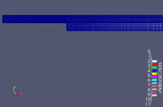
b. Preassure profile.
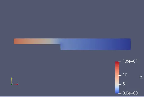
c. Velocity profile.
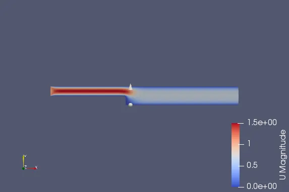
d. Variation Velocity and Preassure profile at 0.085 m from the inlet of geometry for grading =
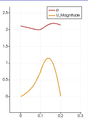
length of Y-axis
Also the values of velocity magnitude max at different grading factors is shown as,
The velocity is maximum at y value of 0.00406, (this is somewhere in the 4th block ie middle of 3rd, 4th &5th block)
0.2- 1.076028 m/s
0.5-1.037318m/s
0.8-1.018488m/s
These are the max velocity magnitude written , the excel sheets are exported from parafoam, in which all the velocity magnitude value are written along with arc length.
Velocity magnitude is square root of the sum of the squares of these velocity components, i.e
√(Vx^2+Vy^2+Vz^2).
The plot for comparison of the three plots looks( near the step region, at 0.085m) like,
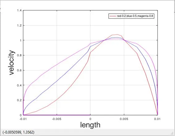
CONCLUSION:
The velocity grows from the walls to the middle of the geometry, the walls resist the flow and so due to shear stress viscous forces are generated. At the walls the velocity is zero i.e the no slip condition. The velocity is maximum at the middle of geometry which is somewhere near the 4 th block if we see for the area near step region.i.e the velocity decreases on both sides of the peak value. This confirms that the plot obtained is correct . The mesh gets finer as the grading factor reduces i.e the 0.2 grading factor has the finest mesh , so the velocity is the most accurate for the simulation when grading factor is 0.2, out of all the three plots although there is not much difference in these three grading factors.