Solving the steady and unsteady 2D heat conduction problem

Aim: To write the code which solves the 2D heat conduction equation by using the point iterative techniques by implementing the following methods.

1. Jacobi

2. Gauss-seidel

3. Successive over-relaxation

Introduction:

Considering General Three dimensional Heat Conduction Equation which has both time derivative and the spatial derivative terms.

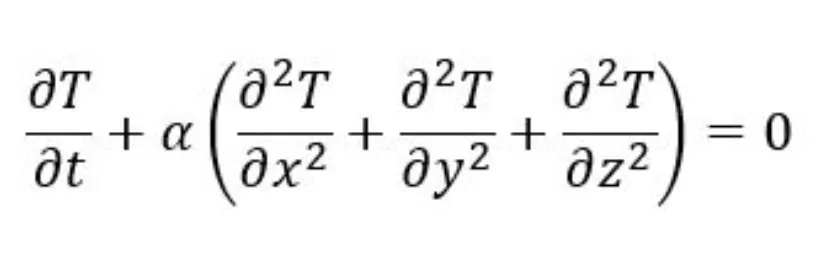
The above equation has 2 terms where term1 represents time derivative and term2 is spatial derivative, where alpha is thermal diffusivity.

Now by considering the assumption that the above equation is solved for a thin plate, dimensions in the Z direction are neglected, thereby the above equation is converted into the following form which is as follows:

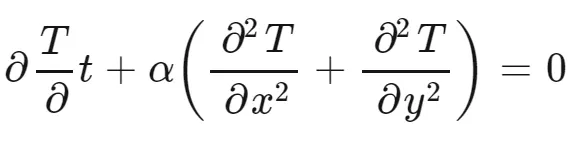
The above equation can be calculated by considering two approaches:

1.Steady State equation:

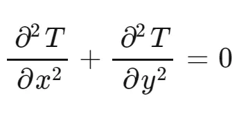
Under these conditions, the rate of change of temperature remains 0. Therefore in this condition time, the derivative term is equated to zero.

Steady-state 2D heat conduction equation:

2.Transient State equation:

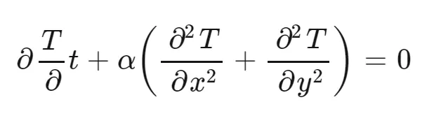
Under these conditions, both terms are considered therefore the equation is as follows:

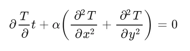
Above two equations can be solved in 2 ways by using 3 iterative methods such as Jacobi, Gauss-Seidel and SOR.

1.Explicit Method

2.Implicit Method

Here in this project Transient state equation is solved by using both ways.

The assumption for solving the problem:

1. Assume that the domain is a unit square.

2. Assume nx = ny=10(for steady ) and 20(for unsteady) [Number of points along the x-direction is equal to the number of points along the y direction]

3. Boundary conditions for steady and transient case

1. Left:400K

2. Top:600K

3. Right:800K

4. Bottom:900K

4.Tolerance=1e-4

5.Starting error=9e9

6.Thermal diffusivity(Alpha)=2.3e-5m^2/sec

7.Doamin length=1m

8.CFL(for stability)=alpha*(dt/(dx^2))

Solving the Steady-state equation:

Considering Two dimensional Steady State Equation

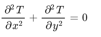
here discretising the equation by applying the central differencing scheme

CODE(steady state):-

clear all
close all
clc
%inputs
nx=10 % number of grid points along x axis
ny=nx ;
x=linspace(0,1,nx);
dx=x(2)-x(1);
y=linspace(0,1,ny);
dy=y(2)-y(1);
z=fliplr(y);
f=1.5;
iter=1;

% Applying BC
t=ones([nx,ny]);

t(1,1:ny)=600;
t(nx,1:ny)=900;
t(1:nx,1)=400;
t(1:nx,ny)=800;
%Temperature at the corner by average value temperature
t(1,1) = (600+400)/2;
t(nx,ny) = (900+800)/2;
t(1,ny) = (600+800)/2;
t(nx,1) = (400+900)/2;

% Creating a copy
told=t;
r1=t;

error=1; %initial error can be assumed to be anything above tolerance
tol=1e-4;
for iterative_solver=1:3
while(error>tol)
for i=2:nx-1
for j=2:ny-1
if(iterative_solver==1)
t(i,j)=jacobi(t,told,i,j);
elseif(iterative_solver==2)
t(i,j)=GS(t,told,i,j);
else
t(i,j)=sor(t,told,i,j,f);
end
end
end
error=max(max(t-told));
told=t;
[u1,v1]=meshgrid(x,z);
%plot

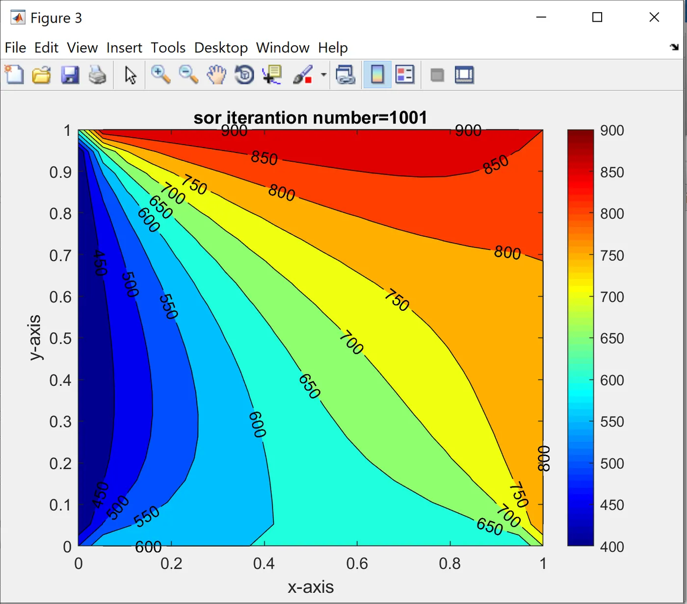
if(iterative_solver==1)
figure (1);
contourf(u1,v1,t);
[C,h]=contourf(u1,v1,t);
colorbar;
colormap(jet);
clabel(C,h);
xlabel('x-axis');
ylabel('y-axis');
title_text=sprintf('jacobi iterantion number=%d',iter);
title(title_text);
pause(0.003);
elseif(iterative_solver==2)
figure (2);
contourf(u1,v1,t);
[C,h]=contourf(u1,v1,t);
colorbar;
colormap(jet);
clabel(C,h);
xlabel('x-axis');
ylabel('y-axis');
title_text=sprintf('GS iterantion number=%d',iter);
title(title_text);
pause(0.003);
else
figure (3);
[C,h]=contourf(u1,v1,t);
colorbar;
colormap(jet);
clabel(C,h);
xlabel('x-axis');
ylabel('y-axis');
title_text=sprintf('sor iterantion number=%d',iter);
title(title_text);
pause(0.003);
end
iter=iter+1;
end
error=1;
iter=1;
t=r1;
told=r1;
end

%function code for jacobi
function out = jacobi(t,told,i,j)
out=0.25*((told(i,j-1)+told(i,j+1)+told(i-1,j)+told(i+1,j)));
end
%function code for GS
function out = GS(t,told,i,j)
out=0.25*(t(i,j-1)+told(i,j+1)+t(i-1,j)+told(i+1,j));
end
%function code for SOR
function out = sor(t,told,i,j,f)
out =((1-f)*told(i,j)+(f*0.25*(t(i,j-1)+told(i,j+1)+t(i-1,j)+told(i+1,j))));
end

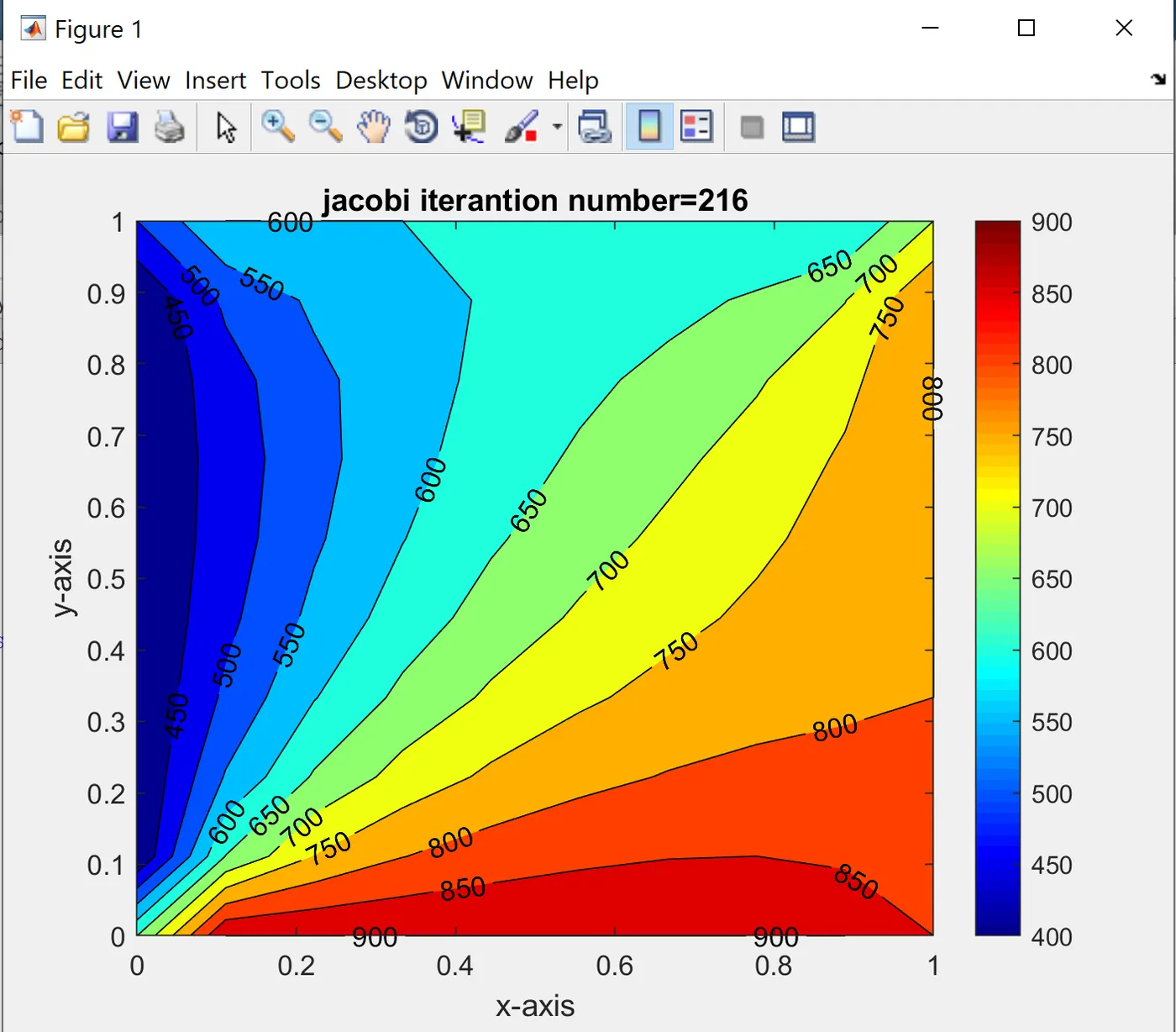
Jacobi:-

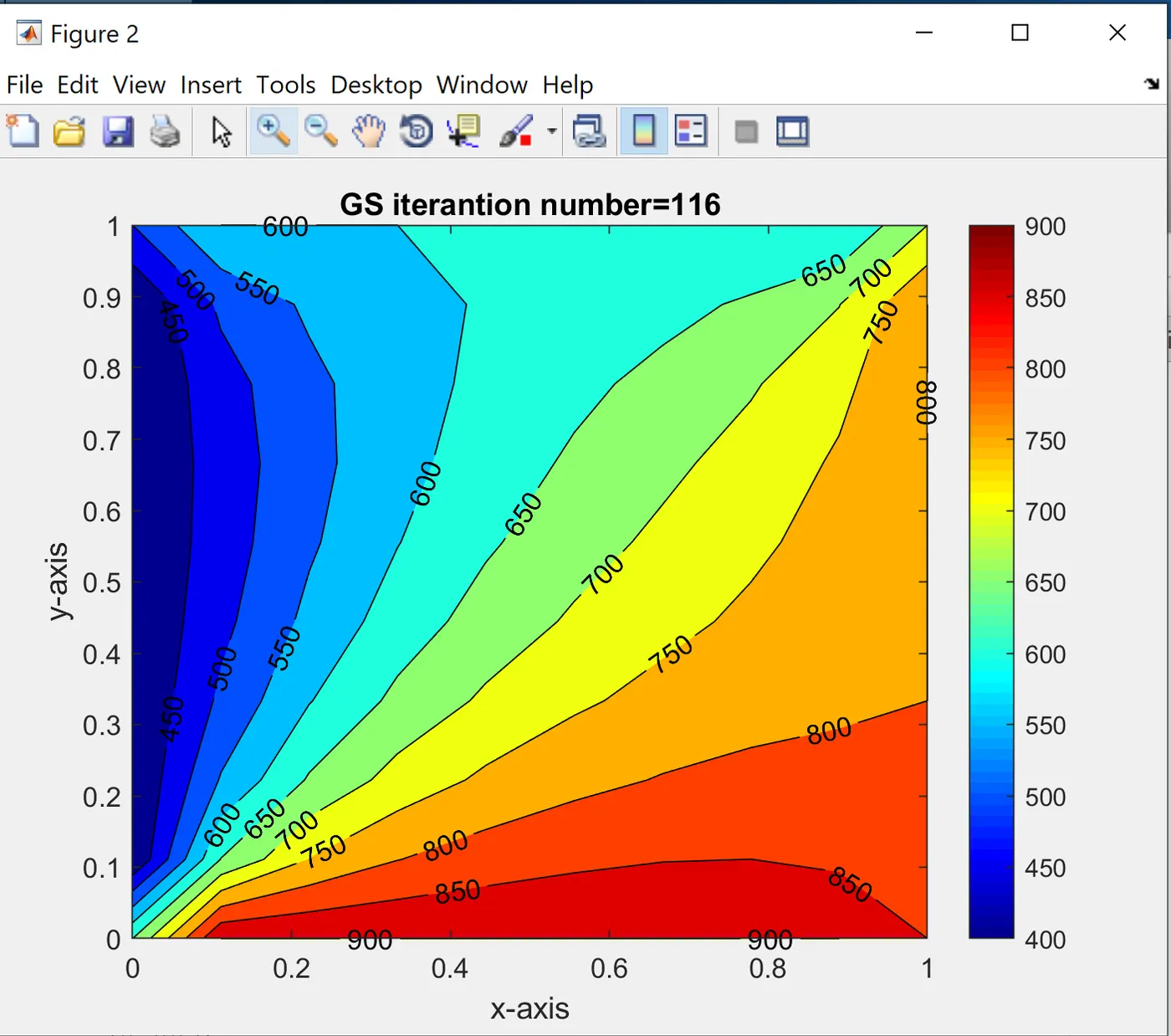
Gauss Seidal:-

SOR Steady State:-

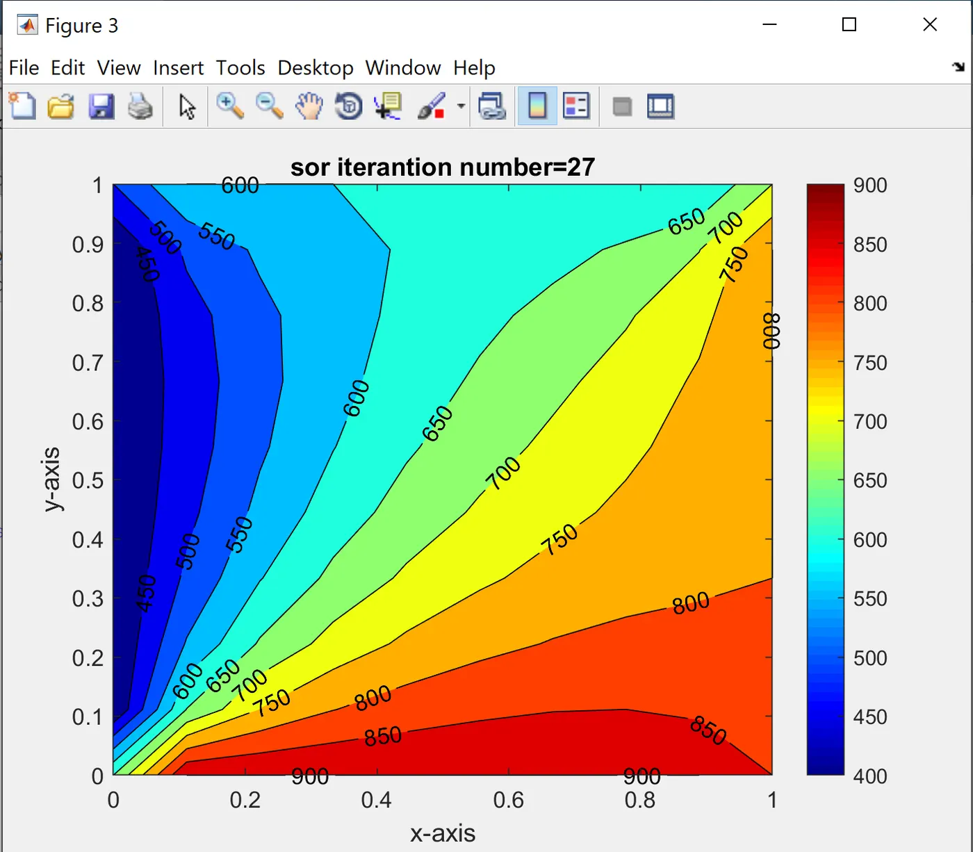
From the all above plots it can be inferred that the SOR method takes less time and less number of iterations when compare to the other two methods. Therefore SOR stands out to be good and fastest among all.

Solving Transient state Equation:

Transient state 2D Steady state heat conduction equation is solved in both ways i.e explicitly and implicitly. Following is the 2D heat conduction equation

Solving the above equation Explicitly:

Explicit Approach is used in numerical analysis for obtaining numerical approximations to the solution of time-dependent ordinary or partial differential equations as in required in computer simulations of a physical process. Explicit methods calculate the state of a system at a later time from the state of the system at the current time.

In this method, each differential equation approach contains only one unknown and can be solved explicitly for this one unknown using this method.

Here in this equation time derivative terms are calculated using the first order differential equations and whereas the term 2 has second-order derivative terms and elliptical in nature so information needs to be taken from all the points equally, So, therefore, a central differencing scheme is applied for the discretising the term2.

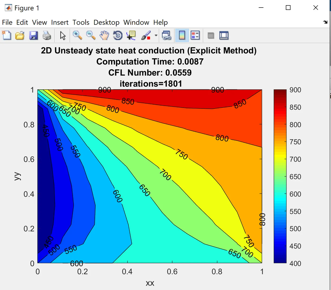
the discretised equation for 2D heat conduction equation for the explicit form is as follows:

CODE for Explicit transient:-

clear all
close all
clc

%basic inputs
nx=10;
ny=nx;
x=linspace(0,1,nx);
dx=x(2)-x(1);
y=linspace(0,1,ny);
dy=y(2)-y(1);

%convective coefficient
alpha=2.3e-5;
tol=1e-4;
%NUMBRER OF TIME STPES
nt=1800;

%TIME STEP
dt=30;

%CFL NUMBER
cfl= (alpha*dt)/dx^2;
k4 = (alpha*dt)/(dx^2);
k5 = (alpha*dt)/(dy^2);
%applying the boundary conditions
t=ones([nx,ny]);
t(1,1:ny)=600;
t(nx,1:ny)=900;
t(1:nx,1)=400;
t(1:nx,ny)=800;

%Temperature at the corner by average value temperature
t(1,1) = (600+400)/2;
t(nx,ny) = (900+800)/2;
t(1,ny) = (600+800)/2;
t(nx,1) = (400+900)/2;

told=t;
[xx,yy]=meshgrid(x,y);
tic % for calculating time taken for ietration
iter=1
for p=1:nt
for i=2:nx-1
for j=2:ny-1
term1 = told(i,j);
term2 = k4*(told(i-1,j)-2*told(i,j)+told(i+1,j));
term3 = k5*(told(i,j-1)-2*told(i,j)+told(i,j+1));
t(i,j) = term1+term2+term3;
end
end

error=max(abs(told-t));
told=t;
iter=iter+1;
end

time=toc; %end time
figure (1);
[C,h]=contourf(xx,yy,t);
colorbar;
colormap(jet);
clabel(C,h);
title(sprintf('2D Unsteady state heat conduction (Explicit Method) n Computation Time: %0.4f n CFL Number: %0.4f n iterations=%d',time,cfl,iter));
xlabel('xx');
ylabel('yy');

Solving the above equation Implicitly:

Implicit Approach is used in numerical analysis for obtaining numerical approximations to the solution of time-dependent ordinary or partial differential equations as in required in computer simulations of a physical process.

Implicit methods find the solution by solving an equation involving both the current state of the system and the later one. Mathematically if Y(t) is the current system state and Y(T+dt) is the state at the later time dt, then, for an explicit method Y(T+dT)=F(Y(t))

Here in this equation time derivative terms are calculated using the first order differential equations and whereas the term 2 has second-order derivative terms and elliptical in nature so information needs to be taken from all the points equally, So, therefore, a central differencing scheme is applied for the discretising the term2.

the final discretised equation for 2D heat conduction equation for the implicit form is as follows:

The above equation is solved iteratively using different iterative methods such as Jacobi, Gauss-Seidel and SOR method.

In Jacobi, the unknowns on the right-hand side are assumed to have an initial value, i.e. T at 'n+1' at all nodes is assumed. Using the equation, then the LHS is calculated. On the next value of i,j similar method is applied to calculate LHS. Thus in the first iteration, value of T for time 'n+1' is calculated at all nodes. The difference between T at 'n+1' which is obtained and T at 'n+1' which was assumed previously is taken. If it is greater than a specified tolerance value, iterations are carried out to calculate T at 'n+1'. But in the second iteration, T at 'n+1' is assumed as the value of T which was obtained in the previous iteration.

Once the value of T is found out iteratively whose error is less than the tolerance value, the value of T is calculated at the next time step 'n+2' using the same iterative method.

Equation for jacobi method are:

term1 = (1+(2*k1)+(2*k2))^(-1);
term2= k1*term1;
term3= k2*term1;
H=(Told(i-1,j)+Told(i+1,j));
v=(Told(i,j-1)+Told(i,j+1));
T(i,j)= (Tprev(i,j)*term1)+term2*H+term3*v

The gauss siedal method is similar to the Jacobi method, but the only difference is- For the first iteration when the value of T at a particular node is calculated, this updated value at that node is used to calculate the value at the next node. But, the error term is calculated similar to Jacobi method, i.e. T at 'n+1' calculated minus the T at 'n+1' previously assumed.

Once the value of T is found out iteratively whose error is less than the tolerance value, the value of T is calculated at the next time step 'n+2' using the same iterative method.

equations for gauss siedal are

term1 = (1+(2*k1)+(2*k2))^-1;
term2= k1*term1;
term3= k2*term1;
H=(T(i-1,j)+Told(i+1,j));
v=(T(i,j-1)+Told(i,j+1));
T(i,j)= Tprev(i,j)*term1+term2*H+term3*v

SOR:

This method can be applied either by using Jacobi or Gauss seidal but the only difference is consideration of factor called omega(scaling factor) which in turn makes the process faster by which the number of iterations required to solve will be decreased

The optimum value of omega is calculated by using the formula:omega=2/(1+sin(pi*dx))

Equations for SOR:

term1 = (1+(2*k1)+(2*k2))^-1;
term2= k1*term1;
term3= k2*term1;
H=(T(i-1,j)+Told(i+1,j));
v=(T(i,j-1)+Told(i,j+1));
T(i,j)= omega*(Tprev(i,j)*term1+term2*H+term3*v)+(1-omega)*Tprev(i,j)

CODE for Transient Implicit Method:-

clear all
close all
clc

%inputs
nx=20;
ny=nx;

x=linspace(0,1,nx);
y=x;
dx=x(2)-x(1);
dy=dx;

% Applying BC
t=ones([nx,ny]);

t(1,1:ny)=600;
t(nx,1:ny)=900;
t(1:nx,1)=400;
t(1:nx,ny)=800;
%Temperature at the corner by average value temperature
t(1,1) = (600+400)/2;
t(nx,ny) = (900+800)/2;
t(1,ny) = (600+800)/2;
t(nx,1) = (400+900)/2;

%defining the value of alpha
alpha=2.3e-5;

%no of time steps
nt=1000;

%storing the time steps in an array

%TIME STPES
dt=30;

%creating the copy
told=t;
t_initial=t;
tprev=t

%defining k1 and k2 (i.e CFL number)
k1=alpha*(dt/dx^2);
k2=alpha*(dt/dy^2);

iterative_solver=1;

error=9e9;
tol=1e-4;

term1=(1+(2*k1)+(2*k2))^(-1);
term2=k1*term1;
term3=k2*term1;
iter=1;
z=cos(pi/nx)+cos(pi/ny); %for SOR
omega = 4/(2+sqrt(4-z^2));
[u1,v1]=meshgrid(x,y);
for iterative_solver=1:3
iter=1;
tic;
for k=1:nt
error=9e9;

while error>tol
for i=2:nx-1
for j=2:ny-1
H=(told(i-1,j)+told(i+1,j));
V=(told(i,j-1)+told(i,j+1));
if iterative_solver==1
t(i,j) =((told(i,j)*term1)+(H*term2)+(V*term3));
elseif iterative_solver==2
t(i,j) =((told(i,j)*term1)+(H*term2)+(V*term3));
elseif iterative_solver==3
t(i,j) =omega*((told(i,j)*term1)+(H*term2)+(V*term3))-(omega-1)*told(i,j);
end
end
end

error_n=max(abs(tprev-t));
error=max(error_n);
tprev=t;

iter=iter+1;

end
told=tprev;
end
%plot
if (iterative_solver==1)
figure (1);
contourf(u1,v1,t);
[C,h]=contourf(u1,v1,t);
colorbar;
colormap(jet);
clabel(C,h);
xlabel('x-axis');
ylabel('y-axis');
title_text=sprintf('jacobi iteration number=%d',iter);
title(title_text);
pause(0.003);
elseif(iterative_solver==2)
figure (2);
contourf(u1,v1,t);
[C,h]=contourf(u1,v1,t);
colorbar;
colormap(jet);
clabel(C,h);
xlabel('x-axis');
ylabel('y-axis');
title_text=sprintf('GS iteration number=%d',iter);
title(title_text);
pause(0.003);
else
figure (3);
[C,h]=contourf(u1,v1,t);
colorbar;
colormap(jet);
clabel(C,h);
xlabel('x-axis');
ylabel('y-axis');
title_text=sprintf('sor iterantion number=%d',iter);
title(title_text);
pause(0.003);

end
time=toc;
fprintf('time taken %i n', time)
end

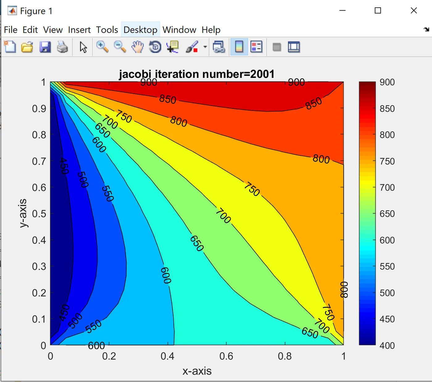
JACOBI:-

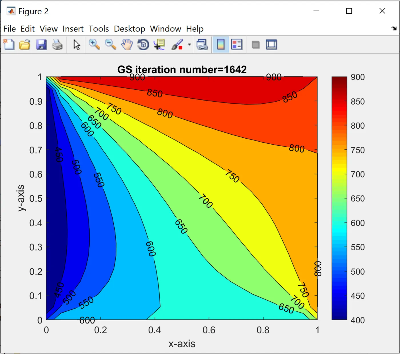
GS:-

SOR:-

time taken for jacobi 1.171323e+00 s
time taken for GS 4.497151e-01 s
time taken for SOR 4.090612e-01 s