Taylor table method using Matlab

1. Central Approximation:

4th order accurate approximation using i-2, i-1, i, i+1 and i+2

Using Taylor series method,

Rewritting in tabular form, we have:

matrix form:-

This is of the form "AX = B". Re-writing them in equation form,

a + b + c + d + e =0 ..........(1)

-2a - b + 0 + d + 2e = 0 ..........(2)

2a + b/2 + 0 + d/2 + 2e = 1 ..........(3)

-4a/3 - b/6 + 0 + d/6 + 4e/6 = 0 ..........(4)

2a/3 + b/24 + 0 + d/24 + 2e/3 = 0 ...........(5)

These equations are solved using MATLAB(inverse matrix multiplication: (A^-1 *B=X)) and the values of a b c d and e are:

a = -0.0833

b = 1.3333

c = -2.5000

d = 1.3333

e = -0.0833

Substituting the values of a b c d and e in taylor series, we get:

2. Skewed Left Approximation:

Using Taylor series method,

In tabular form, we have:

matrix:-

a + b + c + d + e =0 ..........(1)

-4a - 3b - 2c - d + 0 = 0 ..........(2)

8a + 9b/2 + 2c + d/2 + 0 = 1 ..........(3)

-32a/3 - 9b/2 - 4c/3 - d/6 + 0 = 0 ..........(4)

32a/3 + 27b/8 + 2c/3 + d/24 + 0 = 0 ...........(5)

a = 0.9166

b = -4.6666

c = 9.5000

d = -8.6666

e = 2.9166

Substituting the values of a b c d and e in taylor series:

3. Skewed Right Approximation:

4th order accurate approximation using i, i+, i+2, i+3 and i+4

Using Taylor series method,

Rewritting in tabular form, we have:

a + b + c + d + e =0 ..........(1)

0 + b + 2c + 3d + 4e = 0 ..........(2)

0 + b/2 + 2c + 9d/2 + 8e = 1 ..........(3)

0 + b/6 + 4c/3 + 9d/2 + 32e/3 = 0 ..........(4)

0 + b/24 + 2c/3 + 27d/8 + 32e/3 = 0 ...........(5)

a = 1.3396

b = -2.9892

c = 1.9301

d = -0.2508

e = -0.0295

Substituting the values of a b c d and e

CODE:-

clear all
close all
clc

%analytical function = exp(x)*cos(x);
%Creating an INline function
% f = @(x) exp(x)*cos(x);
disp('The analytical function used is = exp(x)*cos(x)')

%taking input for value of x
x =input('Enter the point of approximation ');

% %taking input for calculating dx
max_dx =input('Enter max step size ');
min_dx =input('Enter min step size ');
size =input('Enter interval size ');
dx = linspace(max_dx, min_dx, size);

if (x<max_dx)||(x<min_dx)
error('Invalid Entry');
end

%analytical derivative
%f"(x) = -2*exp(x)*sin(x);
analytical_derivative = -2*exp(x)*sin(x);

for i = 1:length(dx)
central_approximation_error(i) = central_approximation(x,dx(i));
right_skewed_approximation_error(i) = right_skewed_approximation(x,dx(i));
left_skewed_approximation_error(i) = left_skewed_approximation(x,dx(i));
end

figure(1)
loglog(dx,central_approximation_error)
hold on
loglog(dx,right_skewed_approximation_error,'r')
hold on
loglog(dx,left_skewed_approximation_error,'g')
xlabel('Step size, dx');
ylabel('Error');
legend('central approximation error','right skewed approximation error','left skewed approximation error')

%central aprocimation
function out = central_approximation(x,dx)

%analytical function = exp(x)*cos(x);
%f"(x) = -2*exp(x)*sin(x);
analytical_derivative = -2*exp(x)*sin(x);

f = @(x) exp(x)*cos(x);

%calcuation of arbitary constants (a, b, c, d, e) for numerical derivative
syms a b c d e
eqn1 = a + b + c + d + e == 0;
eqn2 = -2*a - b + 0 + d + 2*e == 0;
eqn3 = 2*a + b/2 + 0 + d/2 + 2*e == 1;
eqn4 = -8*a/6 - b/6 + 0 + d/6 + 8*e/6 == 0;
eqn5 = 16*a/24 + b/24 + 0 + d/24 + 16*e/24 == 0;

%Solving Equations to calcualte constants
X = solve([eqn1, eqn2, eqn3, eqn4, eqn5], [a, b, c, d, e]);

%Extracting values of consytants from solution
a = X.a;
b = X.b;
c = X.c;
d = X.d;
e = X.e;

%numerical approximation
central_differencing = (a*f(x-2*dx)+b*f(x-dx)+c*f(x)+d*f(x+dx)+e*f(x+2*dx))/(dx^2);

out = abs(central_differencing - analytical_derivative);

end
%right skew
function out = right_skewed_approximation(x,dx)

%analytical function = exp(x)*cos(x);
%f"(x) = -2*exp(x)*sin(x);
analytical_derivative = -2*exp(x)*sin(x);

f = @(x) exp(x)*cos(x);

%calcuation of arbitary constants (a, b, c, d, e) for numerical derivative
syms a b c d e
eqn1 = a + b + c + d + e == 0;
eqn2 = b + 2*c + 3*d + 4*e == 0;
eqn3 = b/2 + 4*c/2 + 9*d/2 + 16*e/2 == 1;
eqn4 = b/6 + 8*c/6 + 27*d/6 + 64*e/2 == 0;
eqn5 = b/24 + 16*c/24 + 81*d/24 + 256*e/24 == 0;

%Solving Equations to calcualte constants
X = solve([eqn1, eqn2, eqn3, eqn4, eqn5], [a, b, c, d, e]);

%Extracting values of consytants from solution
a = X.a;
b = X.b;
c = X.c;
d = X.d;
e = X.e;

%numerical approximation
right_skewed_differencing = (a*f(x)+b*f(x+dx)+c*f(x+2*dx)+d*f(x+3*dx)+e*f(x+4*dx))/(dx^2);

out = abs(right_skewed_differencing - analytical_derivative);

end
%leftskew
function out = left_skewed_approximation(x,dx)

%analytical function = exp(x)*cos(x);
%f"(x) = -2*exp(x)*sin(x);
analytical_derivative = -2*exp(x)*sin(x);

f = @(x) exp(x)*cos(x);

%calcuation of arbitary constants (a, b, c, d, e) for numerical derivative
syms a b c d e
eqn1 = a + b + c + d + e == 0;
eqn2 = -4*a - 3*b - 2*c - d == 0;
eqn3 = 16*a/2 + 9*b/2 + 4*c/2 + d/2 == 1;
eqn4 = -64*a/6 -27*b/6 - 8*c/6 -d/6 == 0;
eqn5 = 256*a/24 + 81*b/24 + 16*c/24 + d/24 == 0;

%Solving Equations to calcualte constants
X = solve([eqn1, eqn2, eqn3, eqn4, eqn5], [a, b, c, d, e]);

%Extracting values of consytants from solution
a = X.a;
b = X.b;
c = X.c;
d = X.d;
e = X.e;

%numerical approximation
left_skewed_differencing = (a*f(x-4*dx)+b*f(x-3*dx)+c*f(x-2*dx)+d*f(x-dx)+e*f(x))/(dx^2);

out = abs(left_skewed_differencing - analytical_derivative);

end

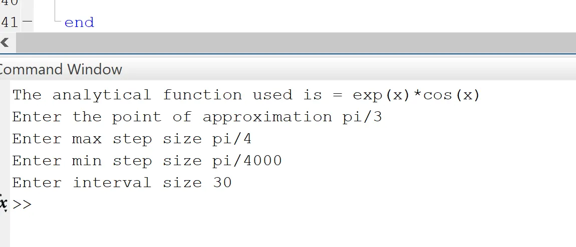
INPUT:-

RESULT:-

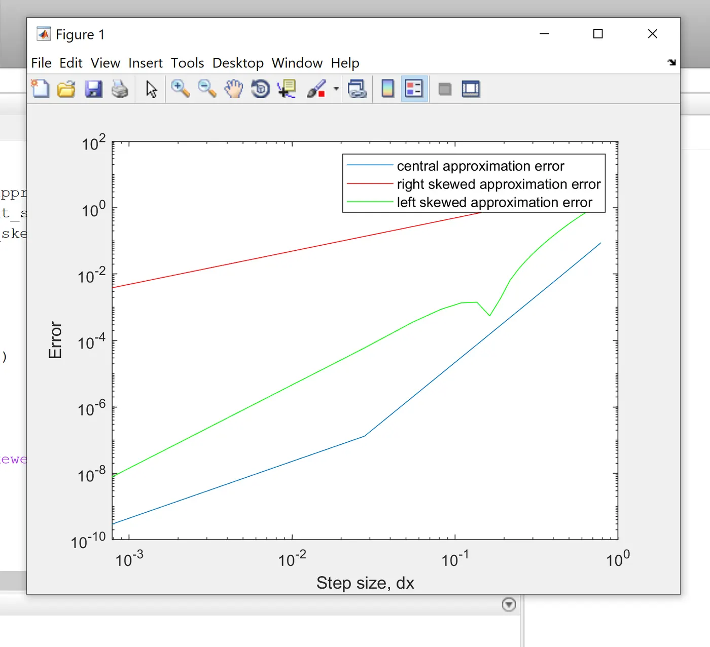
The graph obtained is shown above. From the graph we can clearly understand that Central Approximation Error is less than Left Approximation Error followed by Right Approximation Error. Hence the vartiation of the error is as follows:

Central Approximation Error < Left Approximation Error < Right Approximation Error.

Advantageous of using a skewed scheme over a central differencing scheme:

Skewed schemes are useful for approximating the results on the boundaries of the computational domain This is because, at the boundary of the computational domain node points are available on only one side of the boundary nodes. Central difference schemes demand data from either side of the boundary while the skewed schemes can be configured to take data from only one side of the domain