Simulation of a 1D Super-sonic nozzle flow simulation using Macormack Method
Aim: To compute flow variables for 1D Subsonic Supersonic Flow Nozzle using MacCormack method for conservative and non-conservative equations.
Introduction:
Usually, a numerical solution of the steady, isentropic quasi 1D nozzle flow is redundant because the analytical solution for this problem already exists but the main aim here is to find the solutions for the above flow problem numerically by applying the various CFD techniques which can be supporting evidence for the analytical solution.
Flow which is considered here is the steady, isentropic flow through a convergent-divergent nozzle. The flow at the inlet to the nozzle comes from a reservoir where the pressure and temperature are denoted by p0 and T0 respectively. The cross-sectional area of the reservoir is large and hence the velocity is very small.
The flow is locally subsonic in the convergent section of the nozzle, at the throat section the flow is sonic and then as the area of the nozzle increases the flow gets converted into supersonic at the divergent section.
Normally in reality flow properties vary in both x and y directions, but here in this project, we make the assumption that the flow properties vary only along the x-direction. So, the flow under the assumption is called Quasis one dimensional Flow.
Here the problem is solved with a time-marching solution using Maccormack Method.
figure: Schematic of the subsonic nozzle
MacCormack's Techniques :
MacCormack's Techniques is the explicit finite difference technique which is second-order accurate in both space and time. This method is very effective where we can obtain second-order accuracy with first-order terms and mathematical complexity of calculating the second order time derivative can be avoided.
In this method variable at grid point (i,j) at time t+dt is calculated by using
Here in this time marching is split into two steps i.e predictor and corrected step.
1. Initially, we start with initial conditions.
With the help of initial conditions, we calculate the predictor step.
In this step, the spatial derivatives on the right side are replaced with forward differences.
`(∂ρ/∂x)predictor=(ρ(i+1)-ρ(i))/dx`
With the predicted value of time derivative, we determine the value of 'F' which is called solution update step.
Now this values of the update step are used in the corrected step.
Corrected step:
In the corrected step the spatial derivatives on the right side are replaced with a backward difference.
considering the example of density
Now once after calculating the corrected step, a new time derivative is calculated with the help of both predicted and corrected time derivatives.
Once after calculating the average value, the final solution is obtained with the help of average time derivatives
Governing Equations for 1D Quasi supersonic nozzle flow :
Governing equations are of two types
1.Conservative form.
2.Non-Conservative form.
Non-conservative form of equations:
Continuity:
Momentum:
Energy:
All the above equations consist of non-dimensional variables
Calculation of Time Step:
In this solution magnitude of the time step is calculated based on the Courant number(C). The simple stability analysis of linear hyperbola equations gives that any value of C less than 1 gives a stable solution.
for this problem value of C is considered as 0.5.
The magnitude of dt is calculated by using the formula:
With the help of the above formula, the value of dt is calculated at each every node. Once after calculating the dt value at all the nodes minimum of all dt is considered.
Boundary Conditions:
At the inlet, the flow variables such as temperature and density remain constant and the value of velocity changes.
v1=2*v2-v3
At outlet conditions, all the flow variables keep on changing
Vn=2*Vn-1 - Vn-2
(Rho)n=2*(Rho)n-1 - (Rho)n-2
Tn=2*Tn-1 - Tn-2
Intial Conditions:
Area A = 1 + 2.2*(x-1.5)^2
Density rho=1-(0.3146*x)
Temperature T=1-(0.2314*x)
Velocity v=(0.1+(1.09*x)).*(T.^0.5)
Conservative form of equations:
The equations for Quasis 1D flow are expressed in the generic form.The equations consists of Solution vector U and the flux vector F and the Source term J as follows.
With the help of the above elements, solution vector equations can be written as
Once after solving the above equations our numerical solution will give the results for the solution vector U (U1, U2, U3) in steps of time, this the reason why U is called as Solution vector. In order to obtain the primitive variables density, Velocity, Temperature and pressure Solutions vector must be decoded
Boundary Conditions:
At Inlet boundary conditions the value U1 stays fixed and other two solution vector U2 and U3 will float with respect to time
U2=2*U2-U3;
U3= U1*((T/(gamma-1))+((gamma/2)*(v^2)))
At Outlet boundary conditions the values of solution vector of U1,U2 and U3 will be changing with respect to time.
U1(n)=(2*U1(n-1)-U1(n-2))
U2(n)=(2*U2(n-1)-U2(n-2))
U3(n)=(2*U3(n-1)-U3(n-2))
Intial conditions:
Area A = 1 + 2.2*(x-1.5)^2 it remains constant throughout the nozzle.
Velocity= 0.59/(rho*A)
At t=0, values of density and temperature throughout the nozzle are given as follows
CODE:
Main code
% simulation of 1D super sonic nozzle flow using mccormack method

clear all;
close all;
clc

%taking grid points
n= 31;
x = linspace(0,3,n);
dx= x(2)-x(1);

%A = area
A = 1+2.2*(x - 1.5).^2;
gamma = 1.4;
%time step
nt = 1400;
%coarent number
C = 0.5;
%throat value
throat = ((n+1)/2);

% non conservative form function
tic
[V,rho,T,m,M,P,V_t,rho_t,T_t,m_t,M_t,P_t]= non_conservatine_form(throat,x,gamma,dx,A,n,nt,C);
non_conservatine_form_time = toc;

%conservative form function
tic
[Vc,rhoc,Tc,cons_mass_flow_throat,Mc,pc,Vc_throat,rho_throat,T_throat,cons_mass_flow,Mc_throat,pc_throat]= conservative_form(throat,x,gamma,dx,A,n,nt,C);
conservative_form_time = toc;

%plot for conservative vs non conservative form
%mass flow rate
figure(3)
subplot(3,2,1)
plot(x,m)
hold on
plot(x,cons_mass_flow,'*')
%exact analytical solution is rho*A*V=0.579
plot(x,linspace(0.579,0.579,n),'--')
xlabel('Non dimensional distance of nozzle (x)')
ylabel(' mass flow rate through nozzle (m)')
legend('non conservative form','conservative form','exact analytical solution');
title('comparison of mass flow rate (conventional_form Vs non conv)')
grid on
%variation of non dimensional flow paramenter along x-axis
% mach number
subplot(3,2,2)
plot(x,M)
hold on
plot(x,Mc,'*')
grid on
xlabel('distance of nozzle (x)')
ylabel('Mach number (M)')
legend('non conservative form','conservative form');
title('Mach number profile')

% Pressure
subplot(3,2,3)
plot(x,P)
hold on
plot(x,pc,'*')
grid on
xlabel('distance of nozzle (x)')
ylabel('pressure')
legend('non conservative form','conservative form');
title('Pressure profile')

% density
subplot(3,2,4)
plot(x,rho)
hold on
plot(x,rhoc,'*')
grid on
xlabel('distance of nozzle (x)')
ylabel('density')
legend('non conservative form','conservative form');
title('density profile')

% Temperature
subplot(3,2,5)
plot(x,T)
hold on
plot(x,Tc,'*')
grid on
xlabel('distance of nozzle (x)')
ylabel('TEMPERATURE')
legend('non conservative form','conservative form');
title('Temperature change')

% velocity
subplot(3,2,6)
plot(x,V)
hold on
plot(x,Vc,'*')
grid on
xlabel('distance of nozzle (x)')
ylabel('velocity')
legend('non conservative form','conservative form');
title('velocity profile')

%variation of flow at throat
figure (4)
subplot(4,1,1)
plot(1:nt,rho_throat)
hold on
plot(1:nt,rho_t,'r')
grid on
ylabel('density')
legend('conservative form','non conservative form');
title('density variation at various time step')

subplot(4,1,2)
plot(1:nt,T_throat)
hold on
plot(1:nt,T_t)
grid on
ylabel('temperature')
legend('conservative form','non conservative form');
title('temperature variation at various time step at throat')

subplot(4,1,3)
plot(1:nt,pc_throat)
hold on
plot(1:nt,P_t)
grid on
ylabel('pressure')
legend('conservative form','non conservative form');
title('pressure variation at various time step at throat')

subplot(4,1,4)
plot(1:nt,Mc_throat)
hold on
plot(1:nt,M_t)
grid on
xlabel('time step')
ylabel('mach number')
legend('conservative form','non conservative form');
title('Mach number variation at various time step at throat')
Function for Conservative method:-
% conservative form
function [Vc,rhoc,Tc,cons_mass_flow_throat,Mc,pc,Vc_throat,rho_throat,T_throat,cons_mass_flow,Mc_throat,pc_throat]= conservative_form(throat,x,gamma,dx,A,n,nt,C)
%clear all
%close all
%clc

%input
%L = 3;
%n = 31;
%x = linspace(0,L,n);
%dx = x(2) - x(1);
%gamma = 1.4;
R = 8.314;

%initial conditions
%density and temperature

for i = 1:n

    if(x(i)<=0.5)
        rho_in(i)=1;
        T_in(i)=1;
    elseif (x(i)>0.5)&&(x(i)<=1.5)
        rho_in(i)=1-(0.366*(x(i)-0.5));
        T_in(i)=1-(0.167*(x(i)-0.5));
    else
        rho_in(i)=0.634-(0.3879*(x(i)-1.5));
        T_in(i)=0.833-(0.3507*(x(i)-1.5));
    end

end
%Area
%A = (1+2.2*((x-1.5).^2));
%grid pints for throat
%throat= (n+1)/2;
%velocity
u_in = 0.59./(rho_in.*A);

rhoc = rho_in;
Tc = T_in;
Vc = u_in;

%time steps
%C = 0.5;
dt = 0.0206;
%nt = 1400;
t_sim = (nt- 1)*dt;
t = 0:dt:t_sim;

%initial condition(solution matrix)
U1 = rhoc.*A;
U2 = rhoc.*A.*Vc;
U3 = rhoc.*A.*((Tc/(gamma-1))+(0.5*gamma.*Vc.*Vc));

%U1 = U1_in;
%U2 = U2_in;
%U3 = U3_in;

%Macormack method
for j = 1:length(t)

    %storing ild values
    U1_old =U1;
    U2_old =U2;
    U3_old =U3;
    %flux variables for Predictor step
    F1 = U2;
    F2 = ((U2.^2)./U1) + ((gamma - 1)/gamma).*(U3 - ((gamma/2)*(U2.^2./U1)));
    F3 = ((gamma.*U2.*U3)./U1) - ((gamma*(gamma-1))/2)*(U2.^3)./(U1.^2);

    %predictor method
    for k=2:n-1
         dA_dx(j) = (A(k+1) - A(k))/dx;
         % J2(j) = (1/gamma)*(rhoc*Tc)*dA_dx;
         dlogA_dx = (log(A(k+1))-log(A(k)))/dx;
         J2(k) = dlogA_dx*((gamma-1)/gamma)*(U3(k)-(0.5*gamma*U2(k)^2)/(U1(k)));

         %predictor step
         %contunity equation
         dF1_dx_p = (F1(k+1)-F1(k))/dx;
         dU1_dt_p(k) = -dF1_dx_p;
         %momentum equation
         dF2_dx_p = (F2(k+1)-F2(k))/dx;
         dU2_dt_p(k) = -dF2_dx_p +J2(k);
         %energy equation
         dF3_dx_p = (F3(k+1)-F3(k))/dx;
         dU3_dt_p(k) = -dF3_dx_p;

         %step solution update
         U1(k) = (dU1_dt_p(k).*dt)+U1_old(k);
         U2(k) = (dU2_dt_p(k).*dt)+U2_old(k);
         U3(k) = (dU3_dt_p(k).*dt)+U3_old(k);
    end
     %applying the boundary conditions
     %input
     U1(1) = A(1);
     U2(1) = 2*U2(2)- U2(3);
     U3(1) = U1(1)*((Tc(1)/(gamma-1)+((gamma/2)*Vc(1)^2)));
     %Output
     U1(n) = (2*U1(n-1)) - U1(n-2);
     U2(n) = (2*U2(n-1)) - U2(n-2);
     U3(n) = (2*U3(n-1)) - U3(n-2);

     %calculating primitive variable for corrector term
     rhoc =U1./A;
     Tc = (gamma-1).*((U3./U1)-((gamma/2).*(U2./U1).^2));

     %updating flex variables
     F1 = U2;
    F2 = ((U2.^2)./U1) + ((gamma - 1)/gamma).*(U3 - ((gamma/2)*(U2.^2./U1)));
    F3 = ((gamma.*U2.*U3)./U1) - ((gamma*(gamma-1))/2)*(U2.^3)./(U1.^2);

    %corrector step
   for k=2:n-1
         dA_dx(j) = (A(k) - A(k-1))/dx;
         % J2(j) = (1/gamma)*(rhoc*Tc)*dA_dx;
         dlogA_dx = (log(A(k))-log(A(k-1)))/dx;
         J2(k) = dlogA_dx*((gamma-1)/gamma)*(U3(k)-(0.5*gamma*U2(k)^2)/(U1(k)));

         %predictor step
         %contunity equation
         dF1_dx_c = (F1(k)-F1(k-1))/dx;
         dU1_dt_c(k) = -dF1_dx_c;
         %momentum equation
         dF2_dx_c = (F2(k)-F2(k-1))/dx;
         dU2_dt_c(k) = -dF2_dx_c +J2(k);
         %energy equation
         dF3_dx_c = (F3(k)-F3(k-1))/dx;
         dU3_dt_c(k) = -dF3_dx_c;

   end
   for pc = 2:n-1
       dU1_dt_avg(pc) = 0.5*(dU1_dt_c(pc) +dU1_dt_p(pc));
       dU2_dt_avg(pc) = 0.5*(dU2_dt_c(pc) +dU2_dt_p(pc));
       dU3_dt_avg(pc) = 0.5*(dU3_dt_c(pc) +dU3_dt_p(pc));

       %final update for U1 U2 and U3
       %values before the start of time step
       U1(pc)=(dU1_dt_avg(pc)*dt) + U1_old(pc);
       U2(pc)=(dU2_dt_avg(pc)*dt) + U2_old(pc);
       U3(pc)=(dU3_dt_avg(pc)*dt) + U3_old(pc);
   end
   %applying the boundary conditions
     %input
     U1(1) = A(1);
     U2(1) = 2*U2(2)- U2(3);
     U3(1) = U1(1)*((Tc(1)/(gamma-1)+((gamma/2)*Vc(1)^2)));
     %Output
     U1(n) = (2*U1(n-1)) - U1(n-2);
     U2(n) = (2*U2(n-1)) - U2(n-2);
     U3(n) = (2*U3(n-1)) - U3(n-2);

     %recalculating values
     rhoc=U1./A;
     Vc=U2./U1;
     Tc = (gamma-1).*((U3./U1)-((gamma/2).*(Vc.^2)));

  %pressure ratio
  pc= rhoc.*Tc;
  %mach number
    Mc = Vc./(Tc.^0.5);

    %mass flow rate
    cons_mass_flow = rhoc.*Vc.*A;
    %find variables at throat section
    rho_throat(j)=rhoc(throat);
    T_throat(j)=Tc(throat);
    pc_throat(j)=pc(throat);
    Mc_throat(j) =Mc(throat);
    cons_mass_flow_throat(j)=cons_mass_flow(throat);
    Vc_throat(j)=Vc(throat);
    %plotting mass flow rate at different time steps
figure(2)
if  j==50
    plot(x,cons_mass_flow,'b','linewidth',1.5)
    hold on

  elseif j==100
    plot(x,cons_mass_flow,'r','linewidth',1.5)
    hold on
  elseif j==150
    plot(x,cons_mass_flow,'c','linewidth',1.5)
    hold on
  elseif j==200
    plot(x,cons_mass_flow,'g','linewidth',1.5)
    hold on
  elseif j==550
    plot(x,cons_mass_flow,'y','linewidth',1.5)
    hold on
  elseif j==700
    plot(x,cons_mass_flow,'*','linewidth',1.5)
    hold on
  elseif j==1400
    plot(x,cons_mass_flow,'m','linewidth',1.5)
    grid on
end

 end
xlabel('Non dimensional distance through nozzle (x)','fontsize',10)
ylabel('Non dimensional mass flow rate through nozzle x','fontsize',10)
title('variation of mass flow rate (conservative form) along x at different time steps')
legend({'50 time steps','100 time steps','150 time steps','200 time steps','550 time steps','700 time steps','1400 time steps'});
end
Function for Non Conservative method:-
%Non conservative form

function [V,rho,T,m,M,P,V_t,rho_t,T_t,m_t,M_t,P_t]= non_conservatine_form(throat,x,gamma,dx,A,n,nt,C)

%calcualtions
rho = 1 - 0.3146*x;
% T = temperature
T = 1 - 0.2314*x;
%V = velocity
V = (0.1 + 1.09*x).*T.^0.5;

%time derivative
dt = min(C.*(dx./(sqrt(T)+V)));

%outer time loop
for k= 1:nt
    %saving old values
    rho_old = rho;
    V_old =V;
    T_old = T;

    % predictor step
    for j = 2:n-1

        drhodx_p = (rho(j+1)-rho(j))/dx;
        dvdx_p = (V(j+1)-V(j))/dx;
        dtdx_p = (T(j+1)-T(j))/dx;
        dlogA_dx_p =(log(A(j+1)) - log(A(j)))/dx;

        % contunity equation
        drhodt_p(j) = -rho(j)*dvdx_p - rho(j)*V(j)*dlogA_dx_p -V(j)*drhodx_p;

        %momentum equation
        dvdt_p(j) = -V(j)*dvdx_p - (1/gamma)*(dtdx_p + (T(j)/rho(j))*drhodx_p);
        %energy equation
        dtdt_p(j) = -V(j)*dtdx_p - (gamma- 1)*T(j)*(dvdx_p +V(j)*dlogA_dx_p);
        %solution update
        rho(j) = rho(j) + (drhodt_p(j))*dt;
        V(j) = V(j) + dvdt_p(j)* dt;
        T(j) = T(j) + dtdt_p(j)* dt;

    end

    % corrector step
    for j = 2:n-1

        drhodx_c = (rho(j)-rho(j-1))/dx;
        dvdx_c = (V(j)-V(j-1))/dx;
        dtdx_c = (T(j)-T(j-1))/dx;
        dlogA_dx_c =(log(A(j)) - log(A(j-1)))/dx;

        % contunity equation
        drhodt_c(j) = -(rho(j)*dvdx_c) - rho(j)*V(j)*dlogA_dx_c -V(j)*drhodx_c;

        %momentum equation
        dvdt_c(j) = -(V(j)*dvdx_c) - (1/gamma)*(dtdx_c + (T(j)/rho(j))*drhodx_c);
        %energy equation
        dtdt_c(j) = -(V(j)*dtdx_c) - (gamma- 1)*T(j)*(dvdx_c +V(j)*dlogA_dx_c);

    end
    %compute the average time derivative
    dvdt = 0.5* (dvdt_c + dvdt_p);
    drhodt = 0.5*(drhodt_p + drhodt_c);
    dtdt = 0.5*(dtdt_c +dtdt_p);

    for i =2:n-1
    % final solution update
    rho(i) = rho_old(i) + drhodt(i)*dt;
    V(i) = V_old(i) + dvdt(i)*dt;
    T(i) = T_old(i) + dtdt(i)*dt;
    end
% apply the boundary conditions
%inlet boundary
V(1) = 2*V(2) - V(3);
%outlet
V(n) = 2*V(n-1) - V(n-2);
rho(n) = 2*rho(n-1) - rho(n-2);
T(n) = 2*T(n-1) - T(n-2);


%mass flow rate is m
m = rho.*A.*V;

%pressure ratio is P
P = rho.*T;

%mach number M
M = V./sqrt(T);


%values at throat
rho_t(k) = rho(throat);
V_t(k) = V(throat);
T_t(k) = T(throat);
P_t(k) = P(throat);
M_t(k) = M(throat);
m_t(k) = m(throat);

%exact solution
rho_exact = 0.634*ones(1,1400);
t_exact = 0.833*ones(1,1400);
p_exact = 0.528*ones(1,1400);
mach_exact = 1*ones(1,1400);


%plotting mass flow rate at different time steps
figure(1)
if  k==50
    plot(x,m,'b','linewidth',1.5)
    hold on

  elseif k==100
    plot(x,m,'r','linewidth',1.5)
    hold on
  elseif k==150
    plot(x,m,'c','linewidth',1.5)
    hold on
  elseif k==200
    plot(x,m,'g','linewidth',1.5)
    hold on
  elseif k==550
    plot(x,m,'y','linewidth',1.5)
   hold on
  elseif k==700
    plot(x,m,'black','linewidth',1.5)
    hold on
  elseif k==1400
    plot(x,m,'m','linewidth',1.5)
    grid on
end
end

xlabel('Non dimensional distance through nozzle (x)','fontsize',10)
ylabel('Non dimensional mass flow rate through nozzle x','fontsize',10)
title('variation of mass flow rate (non conservative form) along x at different time steps')
legend({'50 time steps','100 time steps','150 time steps','200 time steps','550 time steps','700 time steps','1400 time steps'});
end
RESULTS
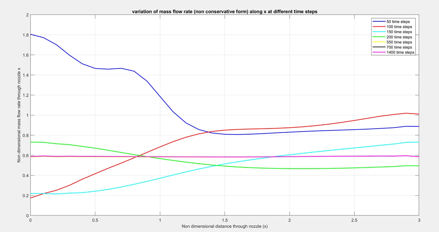
Figure 1 - Shows the variation of mass flow rate at different time steps for non conservative form.
7 different time steps are shown in the graph which depticts different mass flow rate at different time steps.
Mass flow varies from convergent section to divergent section for the earlier time steps. After achieving a steady state which is in between 550 time steps to 700 time steps the variation in mass flow rate also decreases.
We can say that at 700 time steps the value of mass flow rate has been converged.
Plot of conservative form
It shows that at initial time marching as the time derivatives are quite large the mass flow rate values appears to be very high through out the length of nozzle. But after 200 time steps the value is approaching steady state and at 700 time steps we can say that the value is converged. Mass flow rate does not change and remains constant between 700 to 1400 time steps.
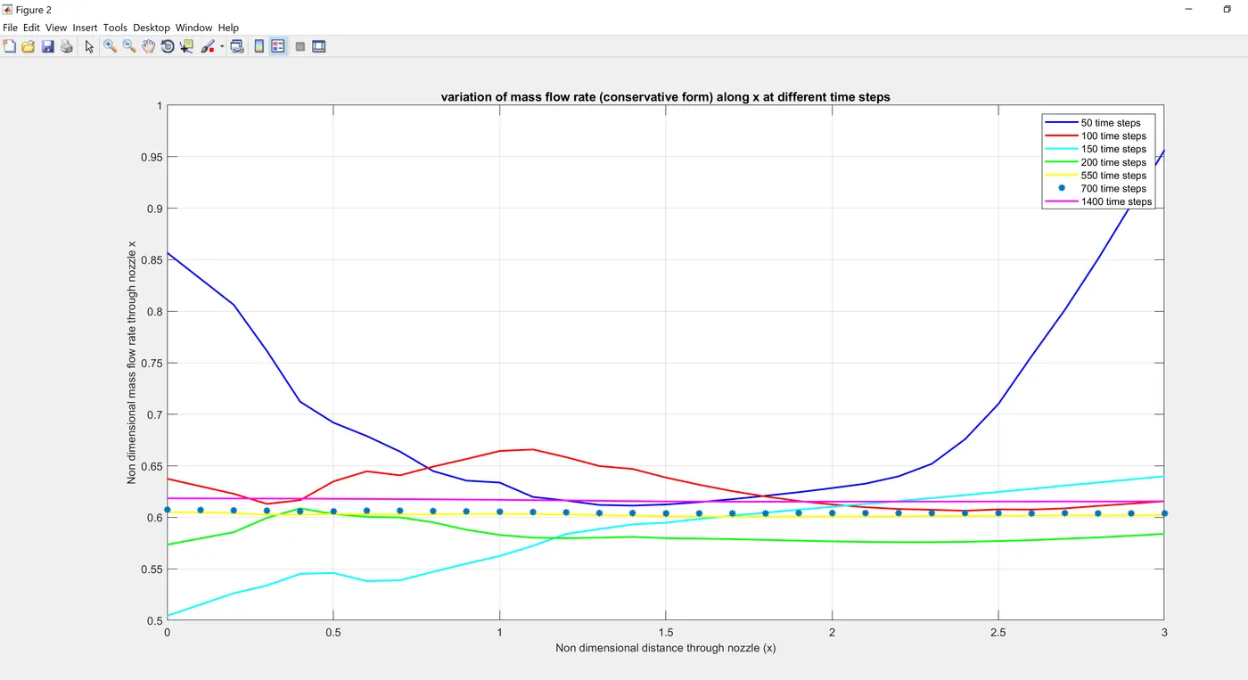
Comparing the mass flow rate variations at different time steps we can say that
1) Conservative form generates better mass flow rate distribution with less fluctuations when compared to non conservative form.
2)The reason is that the mass flow rate is one of the dependent variable in conservative form where as in non conservative form dependent variables are premitive variables.
3) The conservative form generates more accurate results due to flux variables.
Figure 3 (comparison between non conservative and conservative form)
It show that both the forms return identical profile for mach number density velocity pressure and temperature. The mass flow rate is more unstable in non conservative form.
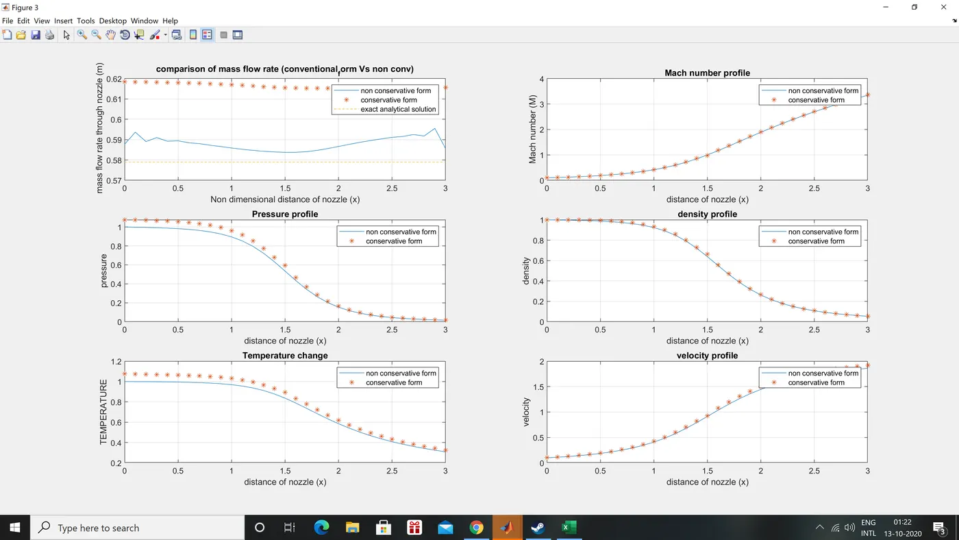
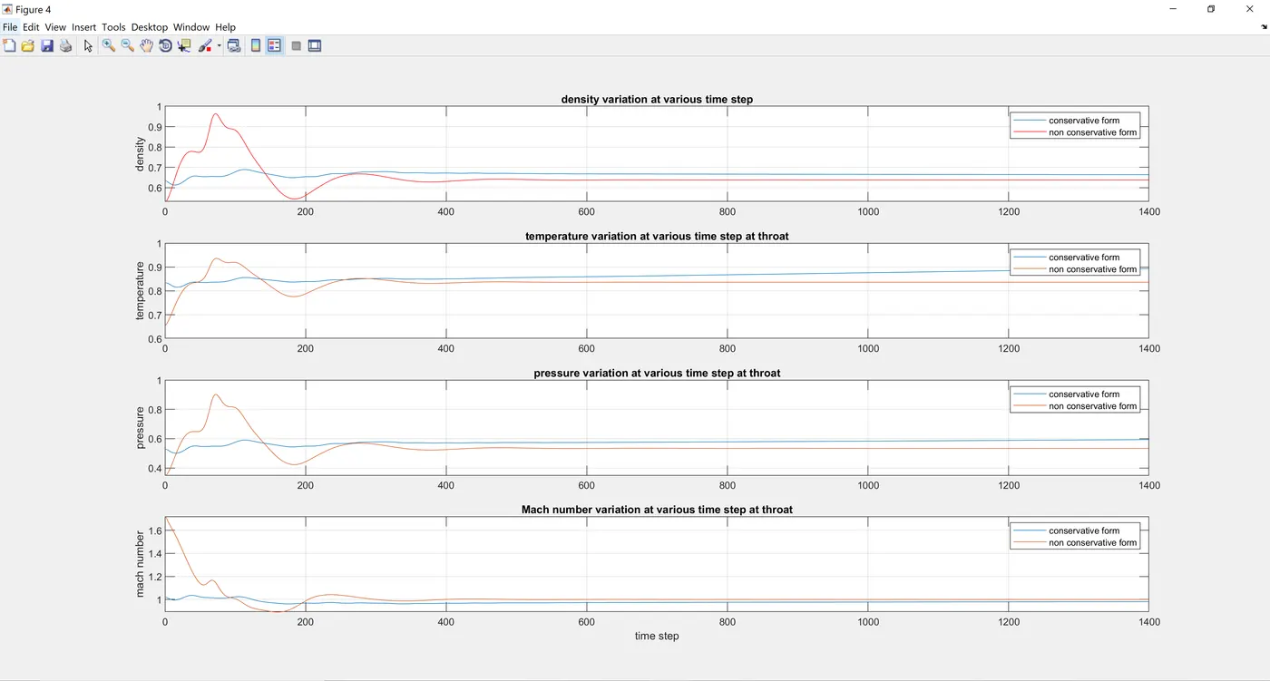
Figure 4 - Convergance paramenter at nozzle throat at different time steps
The graph is plotted for density temperatuer pressure and mach number.
Initially the values of the parameters are high and oscillate, this occures due to various effects on flow shuch as compression and expansion which occures in nozzle.
And in upcoming steps the values are approching near to stability and constant condition.
It can be seen that there are more oscillations occure in 0-200 time steps and gradually decreases from 200-400 time steps.
From the plot we also see that the minimum number of cycles to run is 600 for convergance.
It can be said that the conservative form has less oscillation then non conservative form.
Grid dependance test
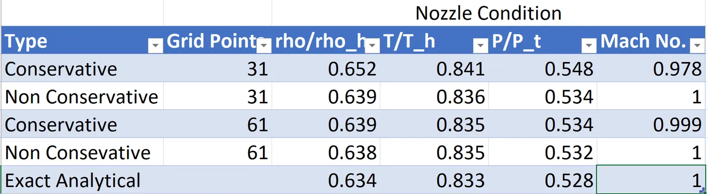
Here rho,T,P represents initial values of pressure temperature and density while rho_t, T_t and P_t represents values at throat.
The two grid points are considered as n =31 and n= 61 while the throat values re taken at i=16
From the table it can be seen that as we increase the number of grid points the value of variables approaches towards exact solution but the change is marginal. But increase in number of grid points increases the run time.
From the results we can also say that non conservative form is slower then conservative form. But if we increase grid points simulation time also increases for both the forms.
Accuracy increases with increased grid points but time for simulation also increases.
Conclusion
1] Simulation time increases with increase in number of grid points but accuracy increases.
2]Non conservative form is faster then conservative form.
3]Mass flow distribution is better in conservative form then in non conservative form as conservative form conserves mass efficiency better.
4]Initially at lower time steps there are oscillations in the solution but as the time steps increases the solution moves to steady state and converges near to 800 time steps.
5]So the simulation must run at least upto 800 time steps for it to converge.
6] Simulation time non -conservative form n=31 is 0.7794 seconds
Simulation time conservative form n=31 is 0.5328 seconds
Simulation time non -conservative form n=61 is 0.7583 seconds
Simulation time conservative form n=61 is 0.7547 seconds
Reference:
Fundamentals of compuational fluid dynamics: https://soaneemrana.org/onewebmedia/COMPUTATIONAL%20FLUID%20DYNAMICS%20BY%20JHON%20D%20ANDERSON2%20JR..pdf