Week 7 State of charge estimation
Aim: To download the file from the link, simulate the 3 test cases from the harness dashboard, and write a detailed report on the results.
To download the file 'CLICK HERE'.
Solution:
--------------- Q1 ---------------
Step-wise solution for opening the file in Matlab
Step 1: After downloading the folder (zip file) into your PC. Extract the file and save it at your convenience.
Step 2: Set the current folder which contains the Battery Management System (BMS) files.
Step 3: Select Battery_System.prj file in the current folder section inside MATLAB,
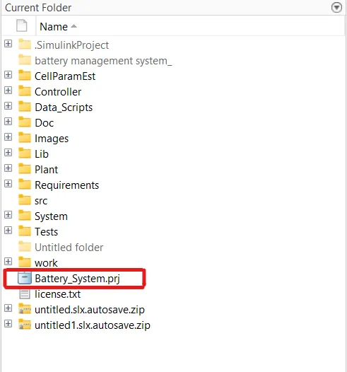
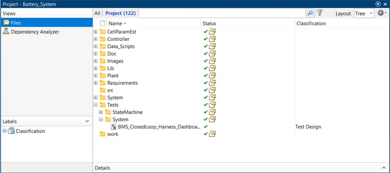
Step 4: After double-clicking the file it will open a window in MATLAB stating Project- Battery_System
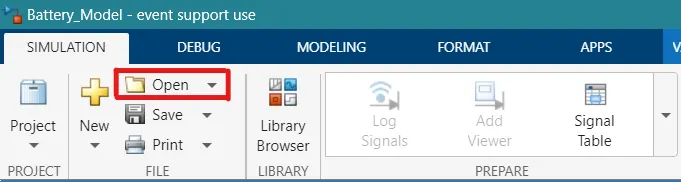
Step 5: To open a model in Simulink, go to
Step 6: Go to the file downloaded path and select plant folder,
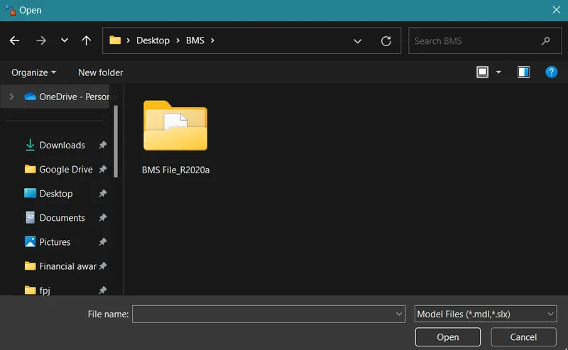
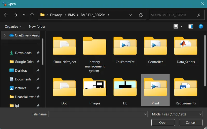
Select the model inside plant folder,
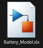
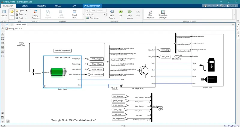
Step 7: Once you open the Simulink model,
Step 8: Go to MATLAB command window and select prj file, double-click the prj file and let the files compute,
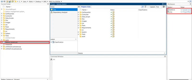
After the files are computed, you will see 2 variables in the MATLAB Workspace, meaning the files are successfully computed.
Step 9: Go to Tests in the MATLAB Command Window, click on the expand file option (Little plus sign before the file titles), Go to Systems and you will observe the files which we need for testing purposes.
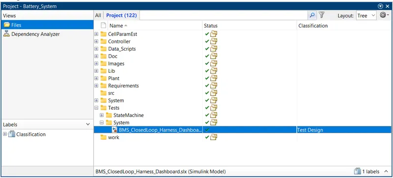
Step 10: Open the model BMS_ClosedLoop_Harness_Dashboard,
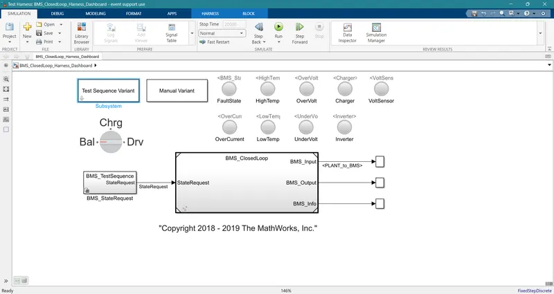
Here we find the information on the dashboard,
Blocks present:
Test Sequence Variant: It is a test sequence selector, the 3 tests we are supposed to simulate in this challenge.
Manual Variant: It is a similar kind of selector as the Test Sequence Variant.
BMS_StateRequest: It is a block that provides BMS_TestSequence (State Request) command as an input to BMS_ClosedLoop Subsystem.
The Lamps: The small cylindrical shaped blocks or lamps are here to indicate the Fault state of the model if there is a concern of High Temperature If the voltage is above the overcharge voltage (Over voltage) and below the cut-off voltage (under voltage) If the charger is plugged in or the temperature is below the suggested temperature.
The Green-colored lamps indicate the good condition and the Red-colored lamps indicate Bad/Faulty conditions.
BMS_ClosedLoop Subsystem:
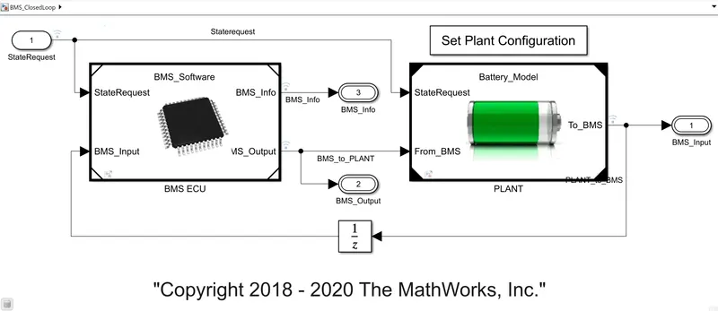
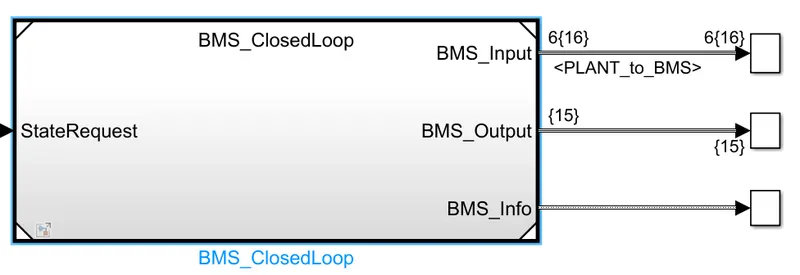
This subsystem contains BMS ECU and PLANT unit.
BMS ECU takes StateRequest and BMS_input as inputs and provides BMS_info and BMS_ouput as outputs.
The plant takes StateRequest and BMS_output as inputs and provides 'BMS_input' as output which is given as input to the BMS ECU unit as a feedback loop.
INSIDE SUBSYSTEMS:
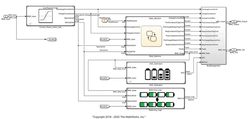
In BMS ECU Subsystem the current power limit calculations are simulated using State Machine Block (Stateflow), SOC estimation, and Cell Balancing logics can be studied.
In the Plant subsystem, we determine the charge load, the pre-charge circuit, and the battery pack is introduced.
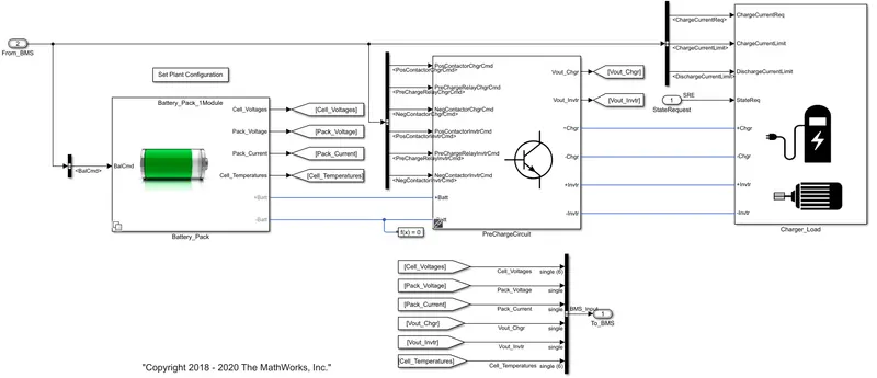
In the battery pack, we have 1 module consisting of 6 cells,
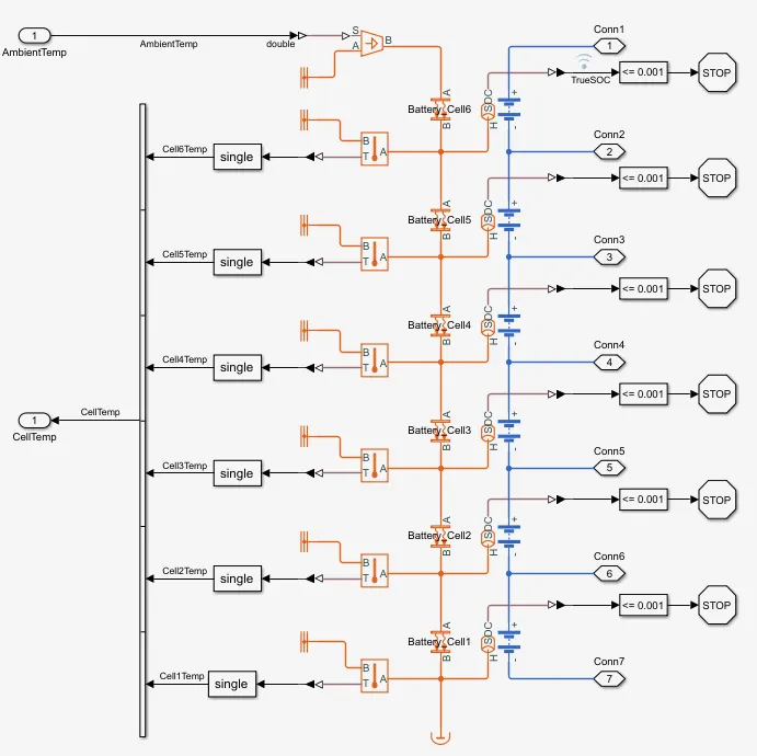
and another module (16 modules) consisting of 96 cells,
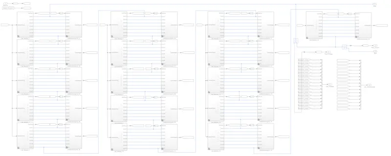
96 cells would take much more time to simulate and run the model, hence, selecting 6 cell configurations.
RUNNING THE MODEL:
For case 1: Go to Test Sequence Variant, and choose 1 as the test case.
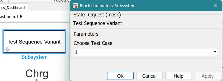
After selecting test case 1, we can observe that the BMS state request now automatically selects test sequence 1 as the model configuration,
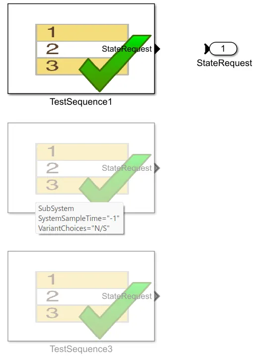
Case 1 would run according to the mentioned sequence inside the TestSequence1 subsystem, i.e.,
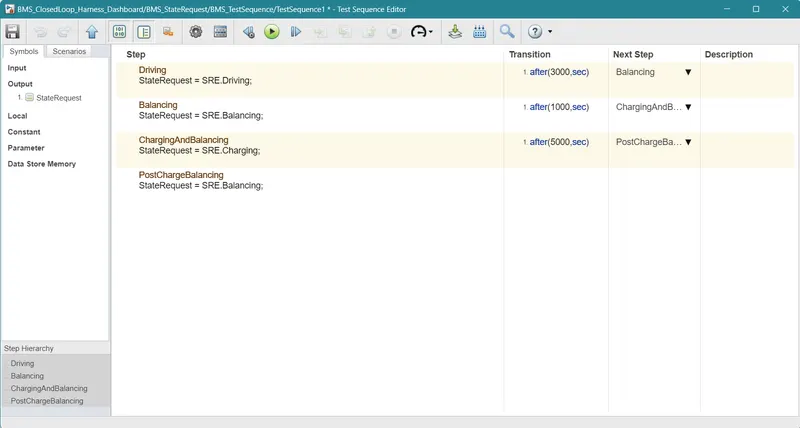
The model will run in driving mode for 3000 seconds, following by which it will start balancing for the next 1000 seconds, and following which the model will then go into the charging mode and also balance the charge inside cells simultaneously for the next 1000 seconds, and finally the post charge operation takes places till the end of the simulation period.
Results and plot discussion:
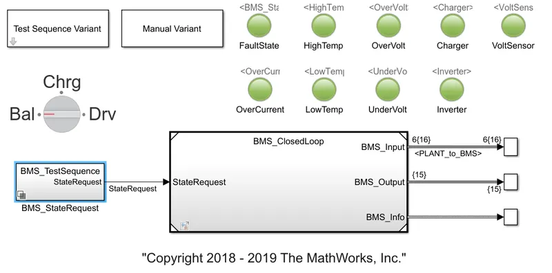
The first check-point of the simulation is to check whether the lamps are indicating any faults in the model or not.
In this case, the lamps are green in color which means the model ran without any faults.
Let's discuss the plot now,
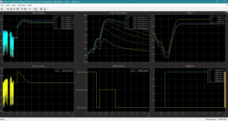
From the plot, we can observe that,
Pack Current and BMS voltage curve:
For the first 3000 seconds, the model (vehicle or cell) is in drive mode where the discharging occurs.
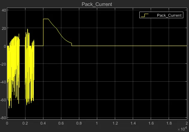
For the next 1000 seconds, the model is on standby mode which means there is no charge and no discharge happening in cells.
In the pack current plot, we can observe that between 1700 seconds to 2000 seconds the cells are on standby mode resulting in the flat line on the graph.
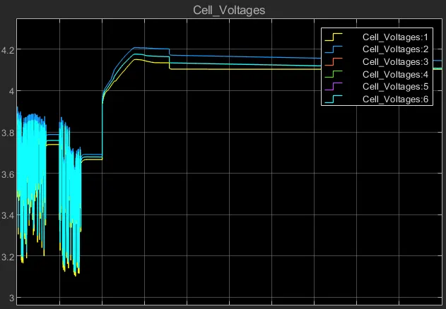
After 4000 seconds the charge mode is on, meaning the cells are in a charging state. BMS voltage increases as the charging state are on. In the BMS voltage graph, we can see that the voltage steeply increases from 3.7V to 3.85V (approximately) and then gradually increases from 4.0V to 4.2V, maximum point (approximately).
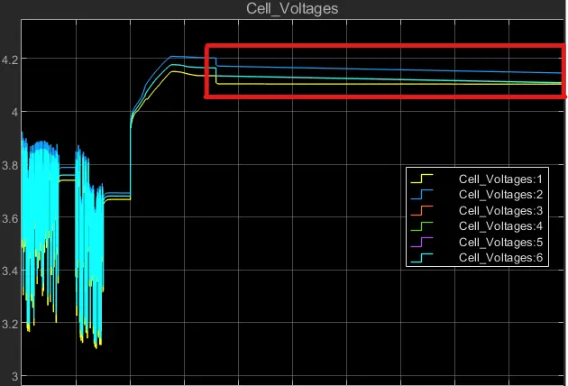
When the voltage reaches 4.2V then the cell balancing takes place in the cells, we can see that all the cell voltages present in the module are merging on 4.1V with a constant flat line indicating that the cells are on standby mode.
As the vehicle is on standby mode, the pack current graph is at rest after 7000 seconds.
Cell temperature curves:
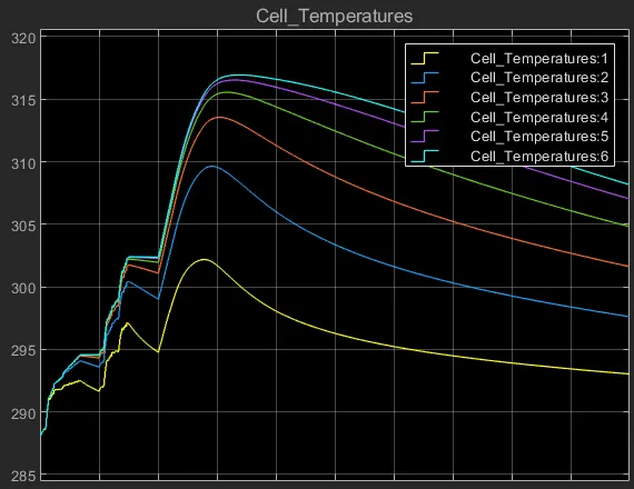
Initially, for 3000 seconds the temperature of cells gradually increases from ambient temperature 288K to 303K. After 3000 seconds up to 4000 seconds, the cell temperatures are decreasing as no current flows through the cell in standby mode. After 4000 seconds temperature starts increasing exponentially up to the constant current region and starts to reduce as current flow reduces in constant voltage and cell balancing region up to 9000 seconds.
The temperature of cell 1 is lesser and cell 6 has a higher temperature for all stages. Cell 1 max temperature raised up to 302K and cell 6 temperature raised up to 317K.
After 9000 seconds the temperatures go on reducing and remain stable after reaching ambient temperature (as the cell is on standby mode there is no increase in temperature curve).
BMS State curve:
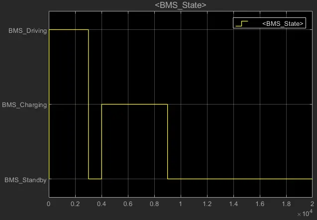
For 3000 seconds the battery module is in drive mode (current is discharging continuously). Between 3000 seconds to 4000 seconds, the battery module is in balancing standby mode as shown in the resulting plot. After 4000 seconds up to 9000 seconds, the battery module is in charging and balancing mode. After 9000 seconds post charge operation takes place till the end of the simulation.
SOC curve:
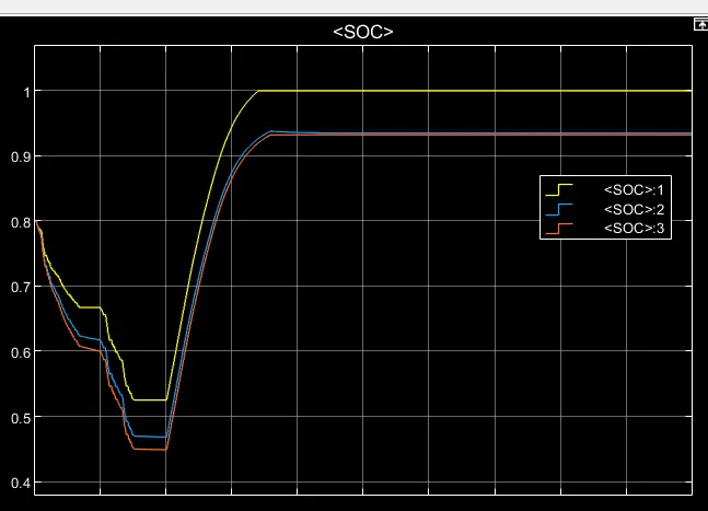
Initially, the SOC of the battery module is at 80%. Here the yellow curve represents SOC estimation done by the coulomb counting technique. The blue curve represents SOC estimation using the Unscented Kalman filter technique. and, the red curve represents SOC estimation using the Extended Kalman filter technique. Among the three UKF and EKF techniques estimate is more accurate than the coulomb counting technique.
For the first 3000 seconds, SOC decreases nearly to 45% during drive mode. After 3000 seconds up to 4000 seconds, the SOC is stable at 45% as cell balancing occurs in standby mode, and between 4000 seconds to 9000 seconds, the module is in charging mode (4000 to 7000 seconds = constant current mode and from 7000 to 9000 seconds = constant voltage mode).
After 9000 secs the SOC becomes stable at approximately 94% as seen from the above plots.
Cell Balancing curve:
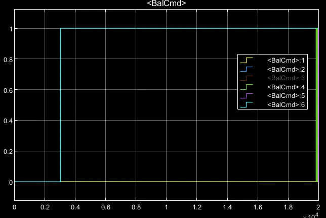
Up to 3000 seconds balancing was not performing. After 3000 seconds cell balancing starts with cell 6 and cell 2 as they raised to 1 state as shown above since its voltage is higher than all other cell voltages. After this stage of charging and balancing, post-charge balancing occurs as cell 6 and cell 2 remain in 1 state till the end of the simulation. As cell 1(yellow) is in lesser voltage than other cells it remains in 0 states throughout the simulation.
For case 2: Go to Test Sequence Variant, and choose 2 as the test case.
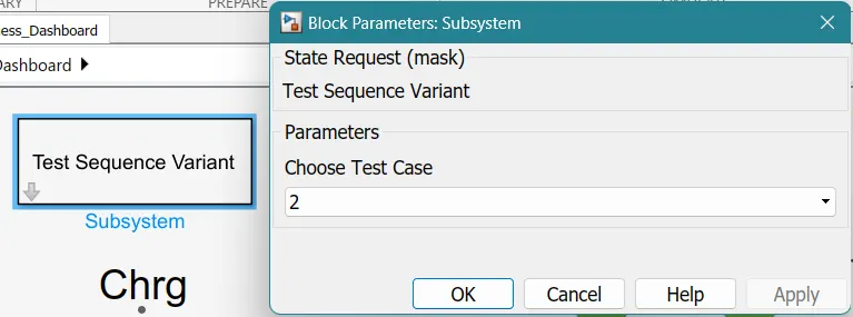
After selecting test case 2, we can observe that the BMS state request now automatically selects test sequence 2 as the model configuration,
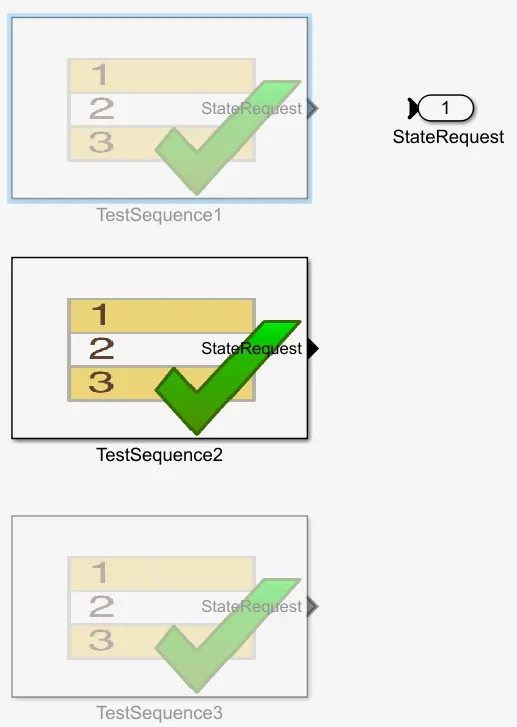
Case 2 would run according to the mentioned sequence inside the TestSequence2 subsystem, i.e.,
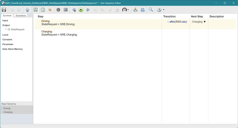
The model will run in driving mode for 5000 seconds, following which the model will then go into charging mode till the end of the simulation period.
Results and plot discussion:
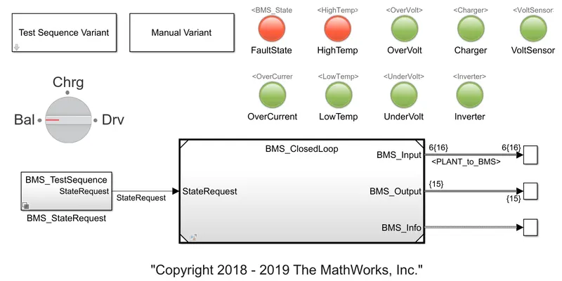
The first check-point of the simulation is to check whether the lamps are indicating any faults in the model or not.
In this case, the cell receives heat resulting in a high-temperature warning and the Fault state is red color, rest of the lamps are green in color which means the model ran without any faults.
Let's discuss the plot now,
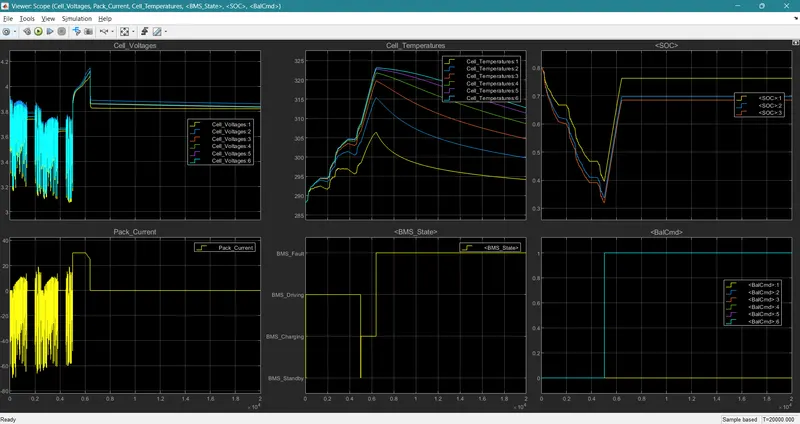
From the plot, we can observe that,
Pack Current and BMS voltage curve:
For the first 5000 seconds(nearly), the model or vehicle or cell is in drive mode where the discharging occurs.
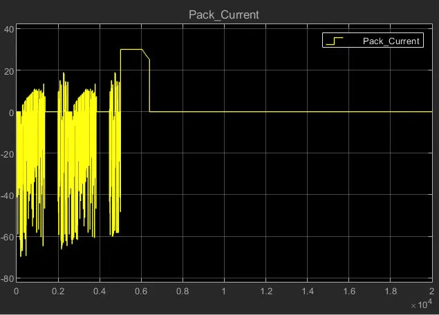
For the next 1000 seconds, the model is on standby mode which means there is no charge and no discharge happening in cells.
In the pack current plot, we can observe that between 1700 seconds to 2000 seconds, also between 3900 seconds to 4200 seconds, the cells are on standby mode resulting in the flat line on the graph.
As the vehicle is on standby mode, the pack current graph is at rest after 6200 seconds (approximately).
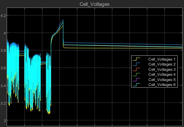
After 5000 seconds the charge mode is on, meaning the cells are in a charging state. BMS voltage increases as the charging state are on. In the BMS voltage graph, we can see that the voltage steeply increases from 3.7V to 3.85V (approximately) and then gradually increases from 4.0V to 4.18V, maximum point (approximately).
When the voltage reaches 4.18V then the cell balancing takes place in the cells, we can see that all the cell voltages present in the module are merging on 3.82V with a constant flat line indicating that the cells are on standby mode.
Cell temperature curves:
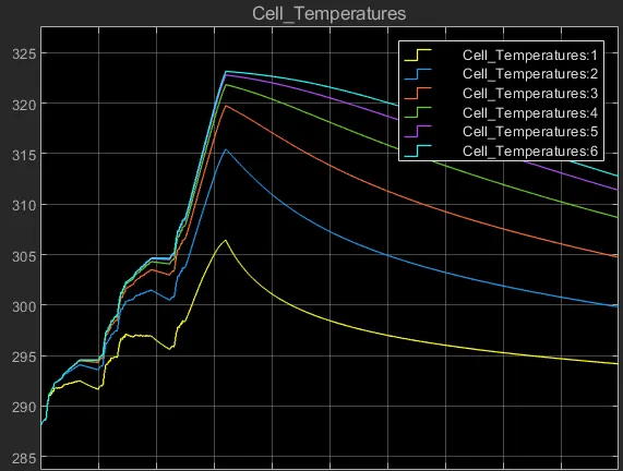
Initially, for 3000 seconds the temperature of cells gradually increases from ambient temperature 288K to 303K. After 4000 seconds up to 5000 seconds, the cell temperatures are decreasing as no current flows through the cell in standby mode. After 5000 seconds temperature starts increasing exponentially up to the constant current region and starts to reduce as current flow reduces in constant voltage and cell balancing region up to 6200 seconds.
The temperature of cell 1 is lesser and cell 6 has a higher temperature for all stages. Cell 1 max temperature raised up to 302K and cell 6 temperature raised up to 321K.
After 9000 seconds the temperatures go on reducing and remain stable after reaching ambient temperature (as the cell is on standby mode there is no increase in temperature curve).
BMS State curve:
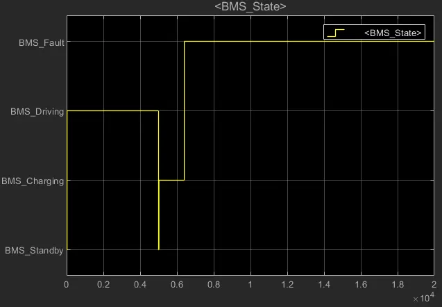
For 5000 seconds the battery module is in drive mode (current is discharging continuously). After 6200 seconds the cell starts to charge, and after 6200 seconds up to 9000 seconds, the battery module is in fault state and hence stops modulating.
SOC curve:
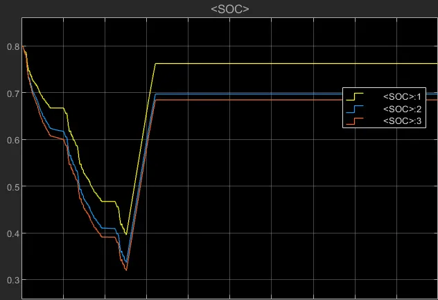
Initially, the SOC of the battery module is at 80%. Here the yellow curve represents SOC estimation done by the coulomb counting technique. The blue curve represents SOC estimation using the Unscented Kalman filter technique. and, the red curve represents SOC estimation using the Extended Kalman filter technique. Among the three UKF and EKF techniques estimate is more accurate than the coulomb counting technique.
For the first 5000 seconds, SOC decreases nearly to 32% during drive mode. Between 5000 seconds to 6200 seconds, the module is in charging mode (4000 to 62000 seconds = constant current mode and from 6200 to 9000 seconds = constant voltage mode).
After 9000 secs the SOC becomes stable at approximately 75% as seen from the above plots.
Cell Balancing curve:
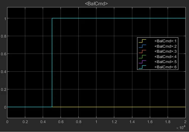
Up to 5000 seconds balancing was not performing. After 5000 seconds cell balancing starts with cell 6 and cell 2 as they raised to 1 state as shown above since its voltage is higher than all other cell voltages. As cell 1(yellow) is in lesser voltage than other cells it remains in 0 states throughout the simulation.
For case 3: Go to Test Sequence Variant, and choose 3 as the test case.
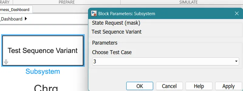
After selecting test case 3, we can observe that the BMS state request now automatically selects test sequence 3 as the model configuration,
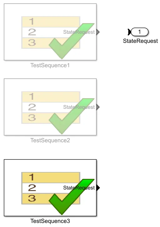
Case 3 would run according to the mentioned sequence inside the TestSequence3 subsystem, i.e.,
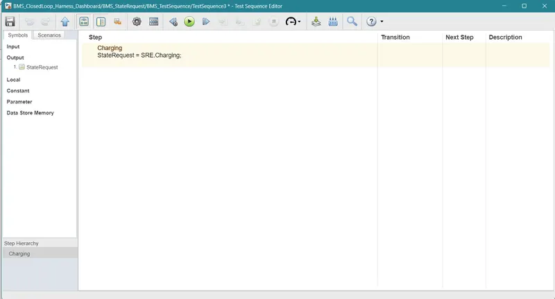
The model will run in charging mode only till the end of the simulation period.
Results and plot discussion:
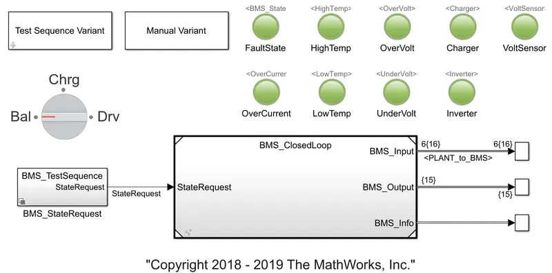
The first check-point of the simulation is to check whether the lamps are indicating any faults in the model or not.
In this case, all the lamps are green in color which means the model ran without any faults.
Let's discuss the plot now,
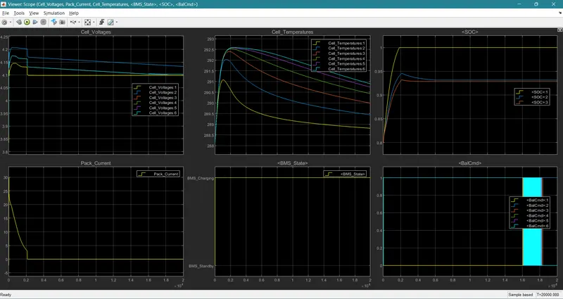
From the plot, we can observe that,
Pack Current and BMS voltage curve:
For the first 5000 seconds(nearly), the model or vehicle or cell is in drive mode where the discharging occurs.
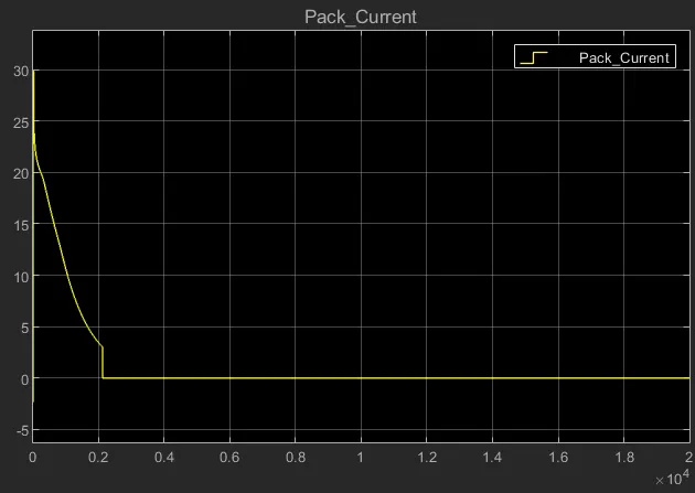
At 0 seconds, the pack current raises from 0 to 30A (Amperes) and after some time, the pack current goes on decreasing up to 2.5A. At 2000 seconds the SOC rests and hence there is a flat line in the graph.
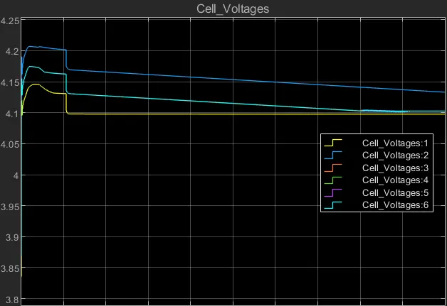
Since the cell is only charging in this case, the voltage drop is not noticed in the graph. Cell number 1 reaches 4.15V and drops down to 4.1V and gets stable throughout the cycle. Cell number 6 (approximately) reaches 4.155V and drops down to 4.145V and Cell number 2 (approximately) reaches 4.21V and drops down to 4.155V
Cell temperature curves:
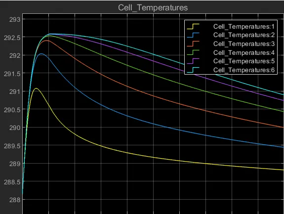
The heat increases inside the cell and hence the temperature of the cell increases gradually from 288K to 292.5K (maximum, approximately) temperature. Cell number 1 reaches its peak temperature at 291K and starts to cool down after 1500 seconds. Cell number 2 reaches its peak temperature at 292K and starts to cool down after 1700 seconds. Cell number 6 reaches its peak temperature at 292.5K and starts to cool down after 2000 seconds.
BMS State curve:
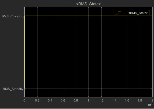
The Battery System is only in charging mode and hence the BMS State directly raises to BMS charging state and stays constant at that state.
SOC curve:
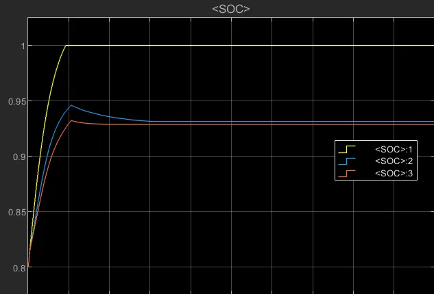
Initially, the SOC of the battery module is at 80%.
The battery pack gets charged in 2000 seconds and the charge remains the same throughout the cycle. The red colored line represents SOC estimation using the Extended Kalman filter technique which is around 93% and the blue colored line represents SOC estimation using the Unscented Kalman filter technique which is around 94%.
Cell Balancing curve:
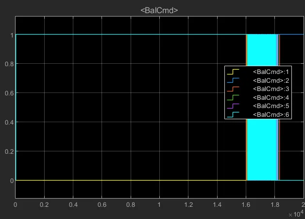
Here, cell number 1 remains at 0 and we can compare other cells with respect to cell number 1, cell numbers 2 and 6 are trying to balance themselves with respect to cell number 1.
--------------- Q2 ---------------
Q. What is coulomb counting? Refer to the above model and explain how BMS implements coulomb counting for SOC estimation?
Solution:
SOC: The SOC of a battery is defined as the ratio of its current capacity (Qt) to its nominal capacity (Qn). The nominal capacity is given by the manufacturer and represents the maximum amount of charge that can be stored in the battery. The SOC can be defined as follows:
`SOC(t) = Qt // Qn`
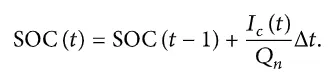
The Coulomb counting method measures the discharging current of a battery and integrates the discharging current over time in order to estimate SOC. The coulomb counting method is done to estimate the SOC(t), which is estimated from the discharging current, I(t), and previously estimated SOC values, SOC(t-1). SOC is calculated by the following equation:
`SOC(t) =SOC (t -1) + I(t) // Qn * ΔT`
But there are several factors that affect the accuracy of the Coulomb counting method including temperature, battery history, discharge current, and cycle life.
Modified Coulomb Counting Method:
To improve the Coulomb counting method, a new technique called the modified Coulomb counting method is proposed. The modified Coulomb counting method uses the corrected current to improve the accuracy of estimation.
The corrected current is the function of discharging current. There is a quadratic relationship between the corrected current and discharging current of the battery. By the practice of experimental data, the corrected current is calculated in the following form:

where, and are constant values obtained from the practice experimental data.
In the modified Coulomb counting method, SOC is calculated by the following equation:
Let's discuss how BMS implements coulomb counting for SOC estimation?
Step 1: Go inside the BMS_ClosedLoop subsystem.
Step 2: Go inside the BMS ECU subsystem.
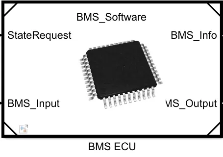
Step 3: Go inside the SOC Estimation subsystem.
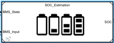
Step 4:
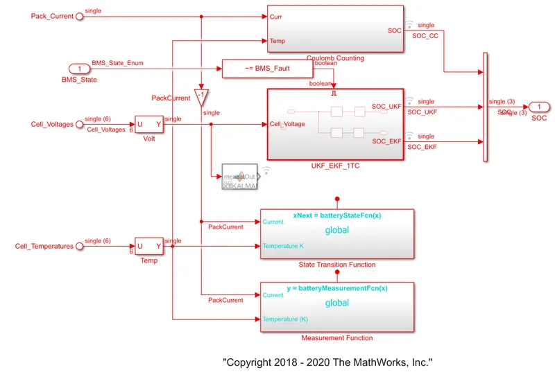
Go to the coulomb counting subsystem: Here we can observe the coulomb counting estimation.
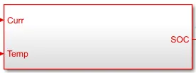
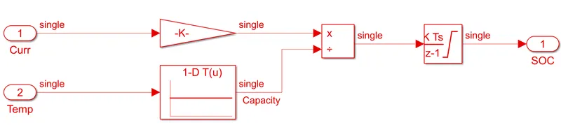
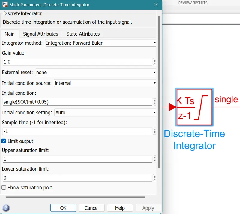
Here the discharge current from the battery is given to gain (single type) with a value of 1/3600 to convert current to Ahr.
The value is divided by capacity due to temperature change. Then integrated with a gain value of 1 with sample time -1 as we are using a discrete integrator.
The saturation limits are from 0 to 1.
We will get the SOC values from 0 to 1 multiplied by 100 to get in the percentage of SOC.
The block Parameters are,
CONCLUSION:
Simulated the 3 test cases from the harness dashboard and discussed a detailed report on the results.
________________________________________________________
ZIP File is provided/attached
________________________________________________________