Project 1 (DHEV)

Aim: To compute the fuel economy numbers for the given vehicle (kmpl) on the urban cycle (UDDS) and highway cycle (HWFET). Also, to analyze and understand the vehicle operation.

Solution:

what is the conventional vehicle?

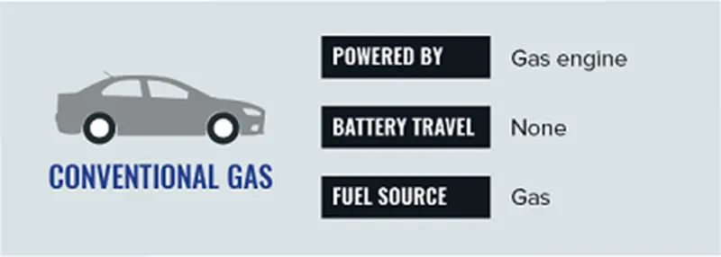
Gasoline and diesel vehicles are similar. They both use internal combustion engines. A gasoline car typically uses a spark-ignited internal combustion engine, rather than the compression-ignited systems used in diesel vehicles. In a spark-ignited system, the fuel is injected into the combustion chamber and combined with air. The air/fuel mixture is ignited by a spark from the spark plug. Although gasoline is the most common transportation fuel, there are alternative fuel options that use similar components and engine systems.

components:

Battery: The battery provides electricity to start the engine and power vehicle electronics/accessories.

Electronic control module (ECM): The ECM controls the fuel mixture, ignition timing, and emissions system; monitors the operation of the vehicle; safeguards the engine from abuse; and detects and troubleshoots problems.

Exhaust system: The exhaust system channels the exhaust gases from the engine out through the tailpipe. A three-way catalyst is designed to reduce engine-out emissions within the exhaust system.

Fuel filler: A nozzle from a fuel dispenser attaches to the receptacle on the vehicle to fill the tank.

Fuel injection system: This system introduces fuel into the engine's combustion chambers for ignition.

Fuel line: A metal tube or flexible hose (or a combination of these) transfers fuel from the tank to the engine's fuel injection system.

Fuel pump: A pump that transfers fuel from the tank to the engine's fuel injection system via the fuel line.

Fuel tank (gasoline): This tank stores gasoline on board the vehicle until it's needed by the engine.

Internal combustion engine (spark-ignited): In this configuration, fuel is injected into either the intake manifold or the combustion chamber, where it is combined with air, and the air/fuel mixture is ignited by the spark from a spark plug.

Transmission: The transmission transfers mechanical power from the engine and/or electric traction motor to drive the wheels.

FORWARD MODEL

The forward model is self-explanatory like forward engineering is a method of creating or making an application with the help of the given requirements and the output is given is the input as in the form of feedback. which let us know how much difference is there between actual and desired values.

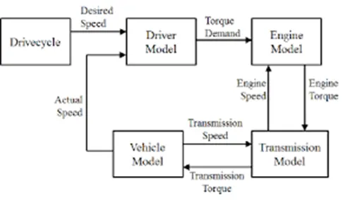
What is a drive cycle?

A drive cycle is typically represented by a series of data points that plots vehicle speed against time. Driving cycles are produced to assess the performance of vehicles in various ways, including fuel consumption and pollutant emissions. Different drive cycles like UDDS, HWFET, FTP, NEDC, etc.

MATLAB Code:

Here we are running the code to load the values and variables so that we can use these values in the Simulink model. This script defines the input values that are required for the calculation.
if else loop is used so that when we change the drive cycle selection values between (1-6) the data of that drive cycle will be loaded.

% Initializing Variable Parameters for Conventional vehicle simulation model
%% Vehicle Parameters

M = 1500; % Vehicle weight [kg]

Cr = 0.015; % Rolling resistance coefficient

Rw = 0.35; % Rolling radius [m]

Cd = 0.33; % Drag coefficient

Af = 2; % Frontal area [m2]

rhoa = 1.225; % Air density [kg/m3]

Vwind = 0; % Wind velocity [kmph]

g = 9.81; % Gravitational acceleration [m/s2]

theta = 0; % Slope [deg]

myu_road_tire = 1; % Coefficient of friction between tire - road interface

%% Powertrain Parameters

FDR = 3.73; % Final Drive Ratio / Diff Ratio

DiffEff = 0.99; % Differential efficiency (assumed independent of operating conditions)

NumGear = 4; % Number of gears in transmission

TransGear = [1:NumGear]; % Transmission Gears

TransRatio = [3.06, 1.62, 1, 0.7]; % Corresponding Transmission ratios

TransEff = 0.90; % Transmission efficiency (assumed independent of operating conditions)

TC_SR = [0, .5, .6, .7, .8, .87, .92, .94, .96, .97, 1]; % Torque Converter Speed Ratio (Matlab default) -> TurbSpd/PumpSpd

TC_TR = [2.232, 1.5462, 1.4058, 1.2746, 1.1528, 1.0732, 1.0192, 1, 1, 1, 1]; % Torque Converter Torque Ratio (Matlab default) -> TurbTrq/PumpTrq

TC_Cf = 1e-4 * [.72558, .66322, .63463, .59042, .51331, .4144, .29287, .22444, .12186, .04386, 0]; % Torque Converter Capacity Factor (Matlab default) -> PumpTrq/PumpSpd^2 [Nm/rpm^2]

load Engine_data_1_9L_Saturn_95kW

load Trans_Shift_map

%% Driver Parameters

Kp = 10; % P gain for driver PI model

Ki = 1; % I gain for driver PI model

Drive_Cycle_Select = 2; % Drive cycle selection

% Drive cycle values in m/s

if Drive_Cycle_Select == 1

load UDDS.mat;

elseif Drive_Cycle_Select == 2

load HWFET.mat;

elseif Drive_Cycle_Select == 3

load FTP.mat;

elseif Drive_Cycle_Select == 4

load US06.mat;

elseif Drive_Cycle_Select == 5

load NEDC.mat;

elseif Drive_Cycle_Select == 6

load WLTP.mat;

end

time_end = cyc_time(end);

vel_end = cyc_vel(end);

Simulink model:

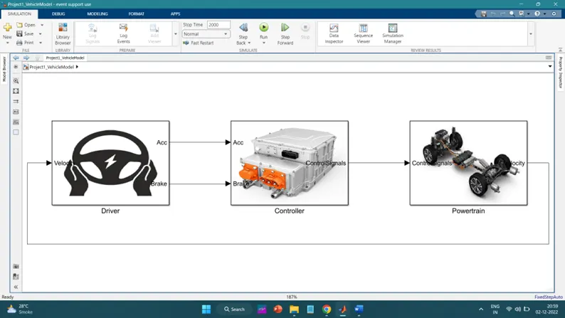
This model consists of 3 main subsystems

• The ‘Driver’ block, is a basic PI controller that generates accelerator and brake pedal outputs to match the desired and actual vehicle speeds.
• The ‘Controller’ block is the brains of the vehicle, representing the electronic control units. Based on the driver inputs, it generates desired engine torque, desired transmission gear, and desired brake torque. These inputs are fed to the ‘Powertrain’.
• The ‘Powertrain’ block represents the drivetrain of the vehicle. It consists of an ‘Engine’ connected to the ‘Automatic Transmission’ through a ‘Torque Converter’. The output of the transmission is connected to the ’Differential’, which powers the ‘Wheels’, which provides the tractive force for vehicle acceleration. The longitudinal dynamics of the vehicle along with the road load is represented in the ‘Vehicle Dynamics’ block which finally gives the velocity, this velocity is given back to the driver block as feedback to check the difference between actual vs desired vehicle speed.
  
  

DRIVER BLOCK:

1-D Lookup Table:

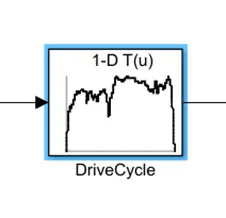
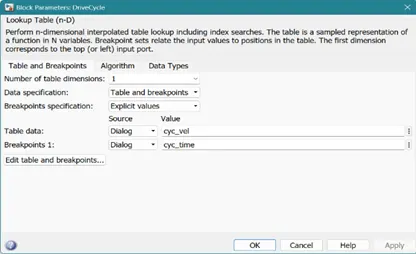
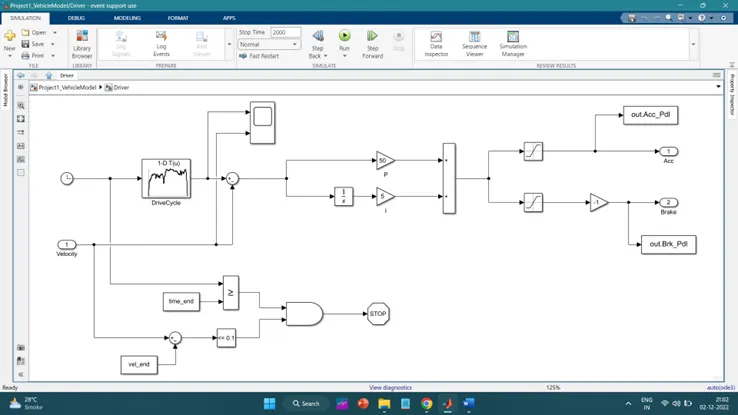
The driver block works on a PI controller. PI controller takes the error and integrates it with a constant and gives the output. Here we have a drive cycle (desired) and velocity (actual) which is vehicle speed for calculating an error. For the drive cycle we are providing time as input and the output of the PI controller is divided into 2 parts and saturated as a positive value for Acceleration and negative values for Brake negative
Besides this, a gain block with a -1 value is used to convert the negative sign of the brake into a positive value.

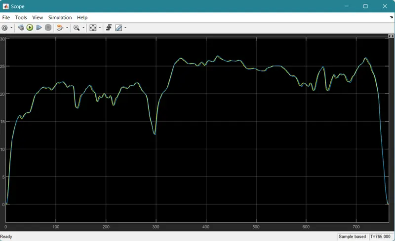
This graph compares the desired and actual velocities.

CONTROLLER BLOCK

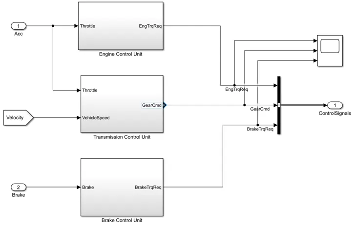
controller block takes acceleration and brake as input and provides Engine Torque, Gear, and Brake Torque as Output. This output is given to Bus Controller to combine all signals into 1 single signal and then by using Bus Selector we can separate all signals present in Bus Controller.

1] Engine Control Unit: First Subsystem of Controller Block

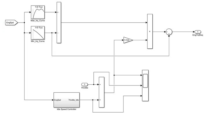
The ideal controller is given so that it does not exceed the ideal speed. The output of the Idle speed controller is then added to the throttle that is received from the driver and based on the maximum and minimum torque curve we calculate the engine torque required.

Idle Speed Controller: Subsystem of Engine Control Unit

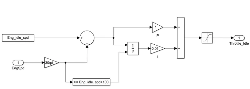
Idle Speed Controller consists of a PI controller where it takes the error of engine ideal speed values (constant) and engine speed value and then calculates the throttle idle by saturating positive values from 0 to 100.

2] Transmission Control Unit: Second Subsystem of Controller Block

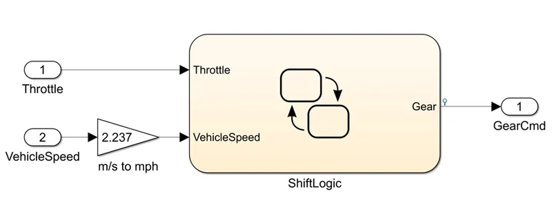
The transmission Control Unit works on State-flow Chart where the inputs given are Throttle and Velocity Speed, giving output as Gear.

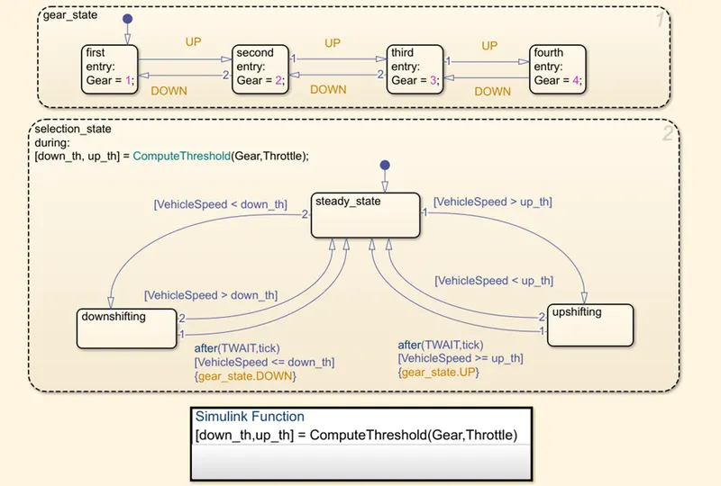
In the Gear Logic system,

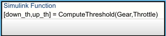
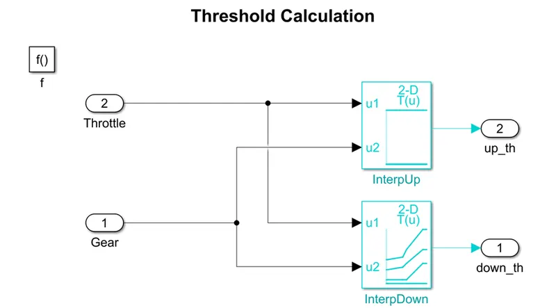
gear state consists of 4 gears which change upon UP and DOWN conditions. These conditions are computed from another state called the selection state, which calls the function which is present in the Simulink function block.

And

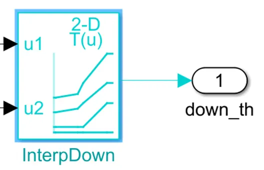
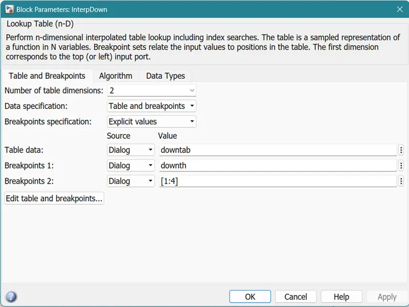
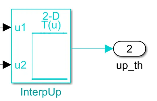
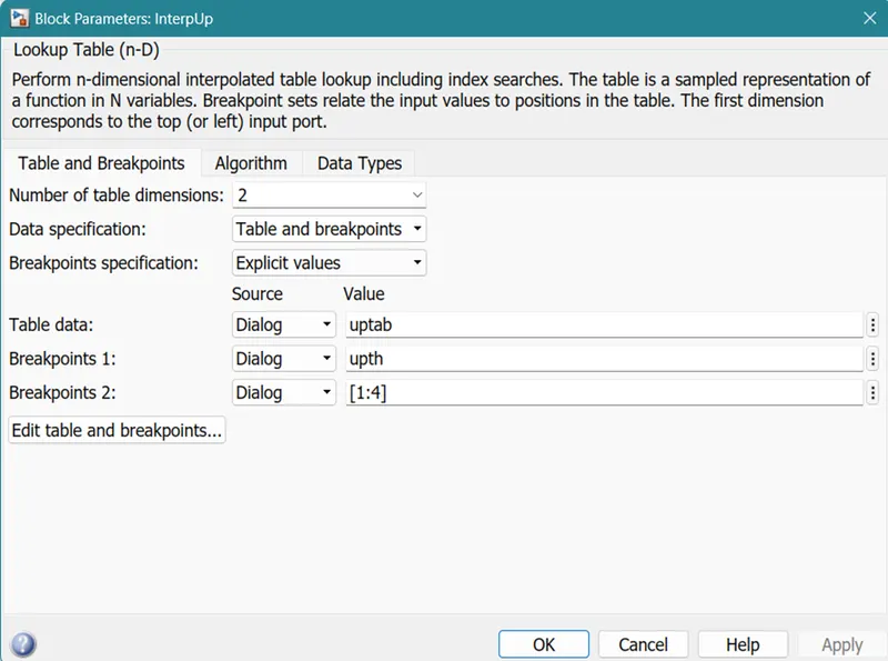
While calculating the Threshold value we give Throttle and Gear as an input to the lookup table and get the gear position values as an output of this block.

3] Brake Control Unit: Third Subsystem of Controller Block

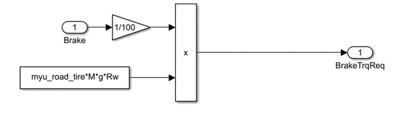
The product of brake and max friction depended on the tire-to-road interface and the weight of the vehicle is calculated for brake torque.

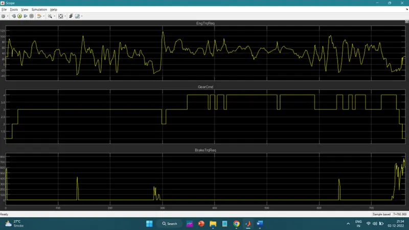
This is the final output of what engine torque is required, the gear selected, and the brake torque.

Power Train Block

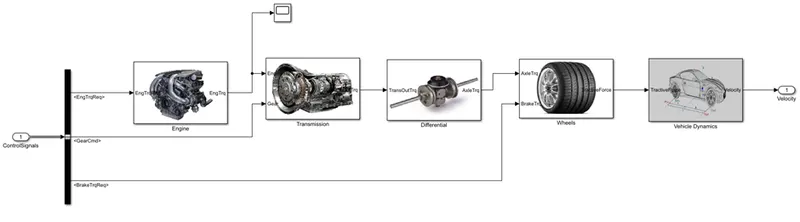
The power train block consists of the engine, transmission, differential, wheel, and vehicle dynamic which are calculated on the basis of torque requirement, Gear ratio, and Break torque.

Engine Subsystem

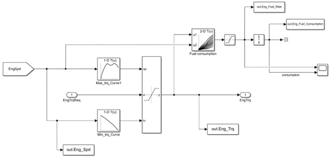
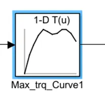
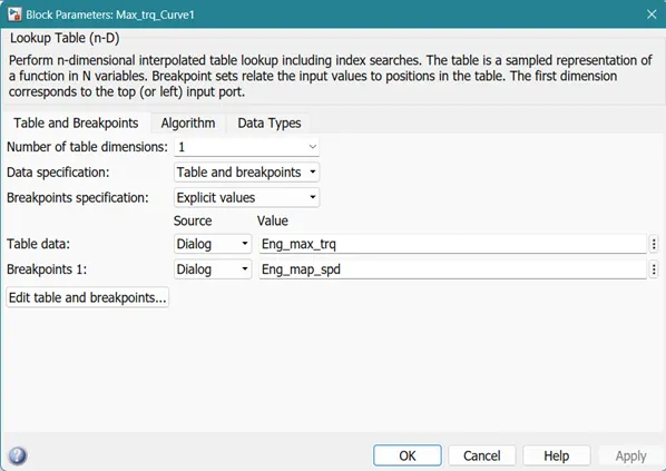
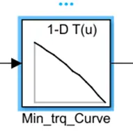
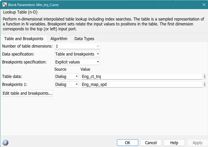
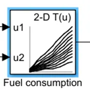
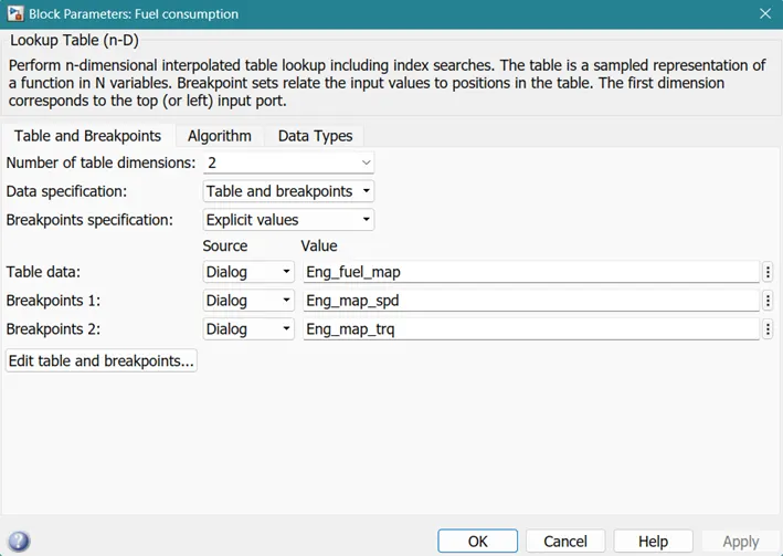
This block is designed to calculate the fuel consumption in the engine at a specific fuel rate on the basis of the torque required. The torque required is checked whether the torque is between the max or min torque curve and then pass it to the fuel consumption map. Based on the speed and torque fuel consumption is calculated and provide the fuel consumption in grams/sec. we are using the To Work-space block to send the values to the MATLAB workspace so that we can use those values for plotting. A saturation block is used to filter the values between the given limit which is 0.5 to -0.5. The integrator is used to convert fuel rate into fuel consumption.

TRANSMISSION

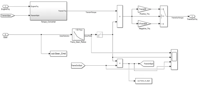
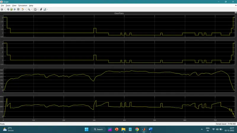
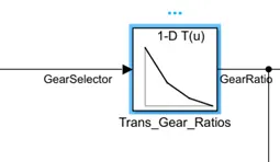
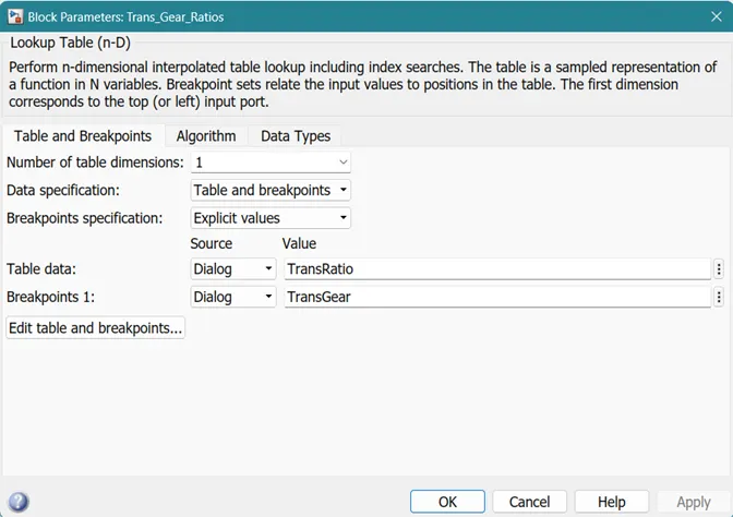
This block takes Engine torque and Gear selector and provides torque output on the basis of gear selector by the driver the gear ratio is filtered from the look-up table.

Scope output:

torque converter

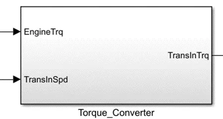
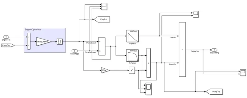
The torque converter is used to connect the engine to the transmission. It also converts the output torque into transmission torque which is multiplied by the gear ratio and given to the switch which on the basis of eff(positive) and loss(negative) provides the output transmission torque.

We are using a torque converter as a fluid coupling device because this system consists of an automatic transmission.

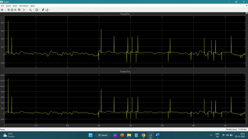
the figure shows the output pump and turbine torque analysis.

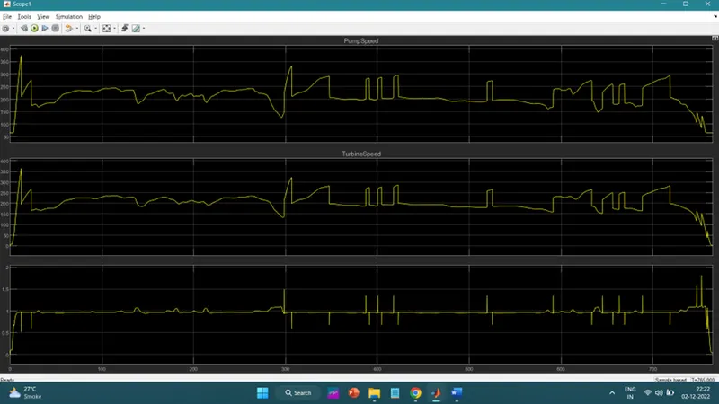
the figure shows the output pump and turbine speed analysis.

DIFFERENTIAL

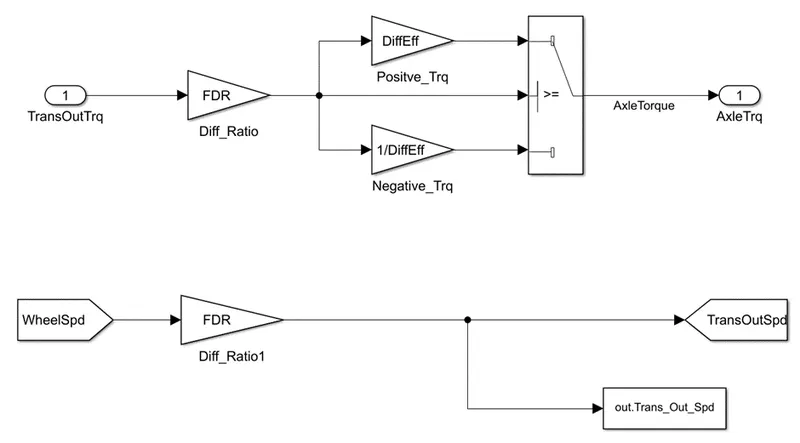
Here we are providing transmission output torque to the differential ratio which gets multiplied and gives the positive and negative values (eff and loss) and passes to the switch which according to the condition gives the output as axle torque. We are using the To Work-space block to send the values to the MATLAB workspace so that we can use those values for plotting.

WHEEL

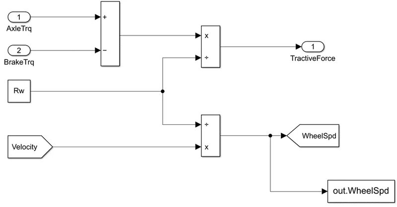
The wheel receives axle torque and subtracts break torque from it and we will get net wheel torque which is divided by the rolling radius to give tractive force. We are assuming here that we have no traction loss for simple calculation.

VEHICLE DYNAMICS

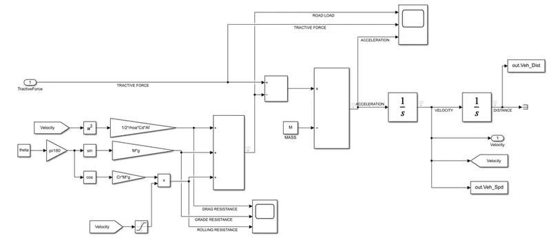
This block is used to calculate the acceleration of the vehicle which is integrated to find velocity followed by distance. Where the input is given as tractive force subtracted by the sum of drag resistance, grading resistance, rolling resistance.

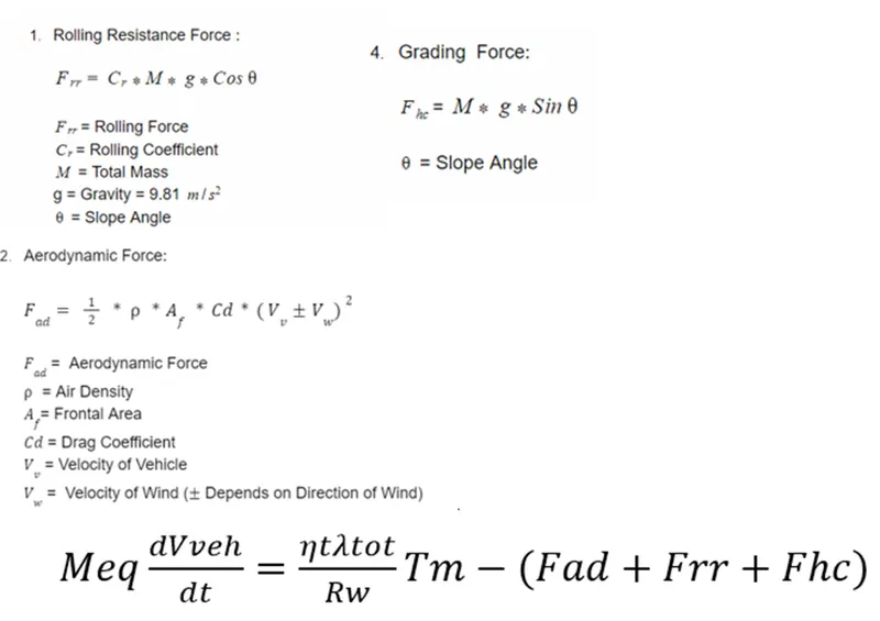
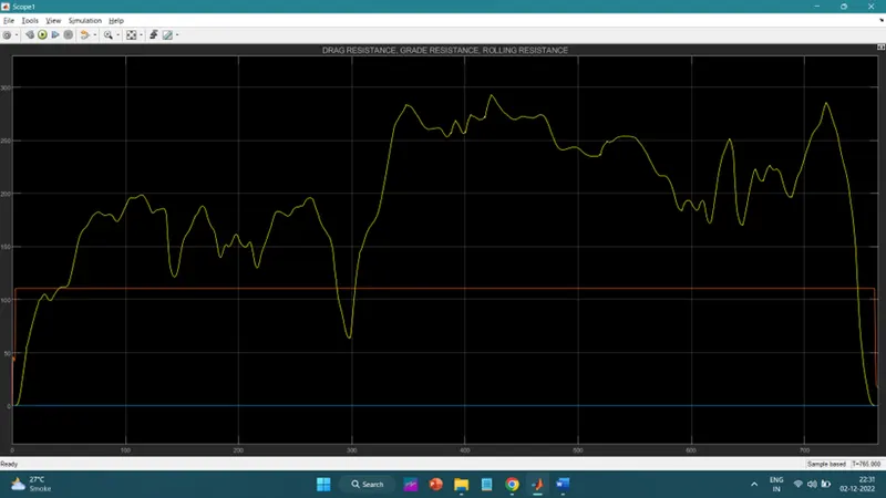
This shows various forces acting in graph.

Post-Processing File

%% Postprocessing File

Time = out.tout;

Acc_Pdl = out.Acc_Pdl; % Accelerator pedal [%]

Brk_Pdl = out.Brk_Pdl; % Brake pedal [%]

Gear_Cmd = out.Gear_Cmd; % Transmission gear

Trans_In_Spd = out.Trans_In_Spd*30/pi; % Transmission input speed [rpm]

Trans_Out_Spd = out.Trans_Out_Spd*30/pi;% Transmission output speed [rpm]

Eng_Trq = out.Eng_Trq; % Engine brake torque [Nm]

Eng_Spd = out.Eng_Spd*30/pi; % Engine speed [rpm]

Eng_Fuel_Consump = out.Eng_Fuel_Consumption; % Engine fuel consumption [g]

Veh_Dist = out.Veh_Dist/1000; % Distance traveled by vehicle [km]

Veh_Spd = out.Veh_Spd*18/5; % Vehicle speed [kmph]

WheelSpd=out.WheelSpd; % wheel speed [rpm]

Eng_Fuel_rate=out.Eng_Fuel_Rate;

%% Data Analysis

Eng_Pwr = Eng_Spd.*pi./30.*Eng_Trq./1000; % Engine brake power [kW]

rho_petrol = 0.7197; % Density of petrol [kg/L]

kmpl = Veh_Dist(end)/(Eng_Fuel_Consump(end)/1000/rho_petrol); % Fuel economy [kmpl]

%% Plotting vehicle characteristics time trace to Engine speed, Engine Torque, Engine Power, And Engine fuel rate, Engine fuel consumption

%% Plotting engine operating points on engine fuel map

figure(1)

hold on; grid on;

plot(Time,Trans_In_Spd, 'linewidth', 1, 'Color', 'black')

plot(Time,Trans_Out_Spd, 'linewidth', 1, 'Color', 'red')

plot(Time,WheelSpd, 'linewidth', 1, 'Color', 'green')

xlabel('time [s]'); ylabel('speed [rpm]');

xlim([0, Time(end)]); ylim([0, 6000]); legend('Trans In Spd','Trans Out Spd','WheelSpd');

%% Plotting torque ,power,fuel rate,fuel consumption

figure(2)

subplot(4,1,1)

grid on;

plot(Time, Eng_Trq, 'linewidth', 1, 'Color', 'black');

xlabel('time [s]'); ylabel('engine torque [Nm]');

xlim([0, Time(end)]);

subplot(4,1,2)

grid on;

plot(Time, Eng_Pwr, 'linewidth', 1, 'Color', 'blue');

xlabel('time [s]'); ylabel('engine power [Nm]');

xlim([0, Time(end)]);

subplot(4,1,3)

grid on;

plot(Time,Eng_Fuel_rate, 'linewidth', 1, 'Color', 'green');

xlim([0, Time(end)]);

xlabel('Time [s]'); ylabel('engine fuel rate');

subplot(4,1,4)

grid on;

plot(Time,Eng_Fuel_Consump, 'linewidth', 1, 'Color', 'red');

xlim([0, Time(end)]);

xlabel('Time [s]'); ylabel('engine fuel consumption');

%% Plotting vehicle characteristics time trace

figure(3)

subplot(4,1,1)

hold on; grid on;

plot(Time, Acc_Pdl, 'linewidth', 1, 'Color', 'black');

plot(Time, Brk_Pdl, 'linewidth', 1, 'Color', 'red'); ylabel('Pedal [%]');

xlim([0, Time(end)]);

legend('Accel','Brake');

subplot(4,1,2)

hold on; grid on;

plot(Time, Gear_Cmd, 'linewidth', 1, 'Color', 'black');

xlim([0, Time(end)]);

xlabel('Time [s]'); ylabel('Gear');

subplot(4,1,3)

hold on; grid on;

plot(cyc_time,(cyc_vel.*(18./5)), 'linewidth', 1, 'Color', 'black');

plot(Time, Veh_Spd, 'linewidth', 1, 'Color', 'red');

ylabel('velocity'); xlabel('Time [s]');

xlim([0, Time(end)]);

legend('desired speed','Actual speed');

subplot(4,1,4)

hold on; grid on;

plot(Time, Veh_Dist, 'linewidth', 1, 'Color', 'black');

xlim([0, Time(end)]);

xlabel('Time [s]'); ylabel('distance [km]');

%% Plotting engine operating points on engine fuel map

figure('Name','Engine Operating Points');

hold on; grid on;

title('Engine Operating Points','fontsize',12);

p1=plot(Eng_map_spd*30/pi,Eng_max_trq,'linewidth',2,'color','r');

p2=line([Eng_map_spd(end)*30/pi Eng_map_spd(end)*30/pi],[0 Eng_max_trq(end)]);

set(p2,'linewidth',1,'linestyle','--','color','k');

p3=line([Eng_map_spd(1)*30/pi Eng_map_spd(1)*30/pi],[0 Eng_max_trq(1)]);

set(p3,'linewidth',1,'linestyle','--','color','k');

[c,h] = contour(Eng_map_spd'*30/pi,Eng_map_trq,Eng_fuel_map');

clabel(c,h);

xlabel('Engine Speed [rpm]'); ylabel('Engine Torque [Nm]');

title('Engine Fuel Consumption Map [g/s]');

p4 = plot(Eng_Spd,Eng_Trq,'.','color','k');

legend([p1 p4],{'Max Curve','Operating Points'});

axis([Eng_map_spd(1)*30/pi Eng_map_spd(end)*30/pi 0 Eng_map_trq(end)]);

In this code, we will plot the values that are extracted from the Simulink model and compare it with {UDDS CYCLE VS HWFET CYCLE}

1. Tabulate the fuel economy numbers (kmpl) for UDDS and HWFET cycles.

fuel economy numbers (kmpl) for UDDS cycle = 16.8534

fuel economy numbers (kmpl) for HWFET cycle = 21.2041

fuel economic number is high in the HWFET cycle since there is low pedaling which causes low energy loss hence less fuel consumption whereas as we see in the UDDS cycle there is more pedaling means more energy loss due to loss which causes more fuel consumption.

2. Plot the time trace for the engine, transmission input, transmission output, and wheel speed on one plot.

In the below figure1 we can see there is more fluctuation in speed which means transmission speed is decreasing to zero with time which generates less energy. But if we compare this in figure 2, we can see that there is less fluctuation in speed which means transmission speed is minimal or almost equal to zero for long period of time which generates more energy. we can see this in figure5 and 6.

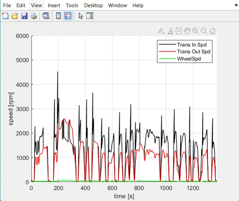Figure 1: Engine, transmission input, transmission output and wheel speed for UDDS cycle.

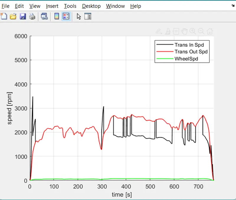Figure 2: Engine, transmission input, transmission output, and wheel speed for HWFET cycle.

3 . Plot engine torque, engine power, fuel rate, and fuel consumption using subplots.

In figure 3 and 4 we can see the engine torque, engine power, and fuel rate is directly proportional to each other, which means as engine power has increased the torque also increased, and at time fuel rate is also increased. The main difference between figures 3 and 4 is fluctuation due to instant increase and decrease in power, torque, and fuel rate it is mainly due to the driving condition.

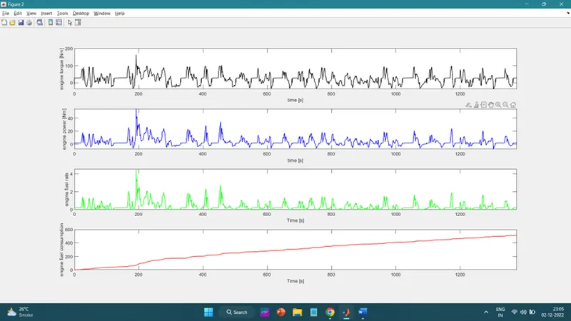Figure 3: Engine torque, engine power, fuel rate, and fuel consumption for the UDDS cycle.

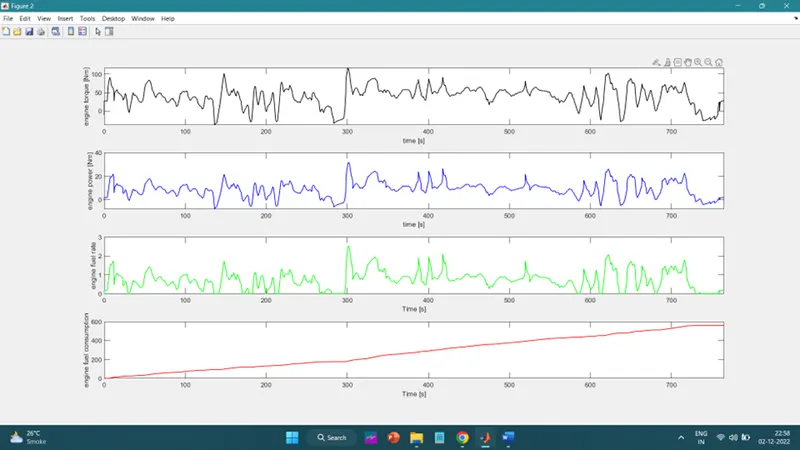Figure 4: Engine torque, engine power, fuel rate, and fuel consumption for the HWFET cycle.

3. Plot accelerator and brake pedal, gear command, vehicle desired and actual speed, and vehicle distance using subplots.

In figure5 we can see that if the gear is not constant for long period, we will receive less velocity whereas in figure6 the gear is stable for a long period which means the velocity is increasing due to which there is less pedaling hence there is a minimal power loss. By looking at graph5 and 6 we can identify that vehicle is making stop-and-go motions multiple times in a given distance due to zero velocity UDDS cycle whereas in the HWFET cycle there is no motion of stop and go, the vehicle’s velocity is fluctuates because the input velocity is such that the vehicle never stops but it reduces speed after a certain period of time and increases its velocity again. This cycle continues as we see in the HWFET cycle.

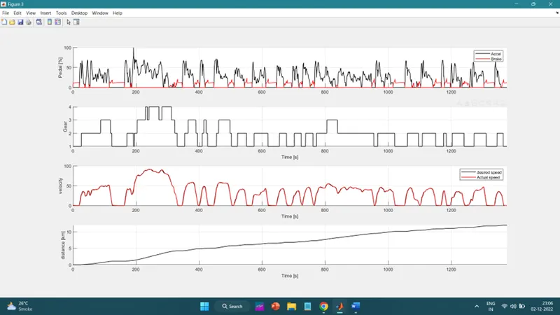Figure 5: Accelerator and brake pedal, gear command, vehicle desired and actual speed, vehicle distance for UDDS cycle.

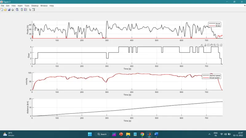Figure 6: Accelerator and brake pedal, gear command, vehicle desired and actual speed, vehicle distance for HWFET cycle.

4. Plot the engine operating points on the engine fuel map.
   
   From the below figures, we can see that in the UDDS cycle engine operating points are exceeding the max curve whereas in the HWFET cycle the engine operating points are low. In both the figures we can see that there is a much higher RPM available that is not used.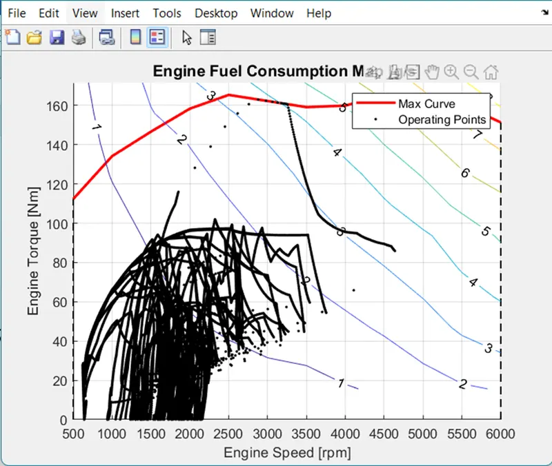 Figure 7: Engine operating points for the UDDS cycle.

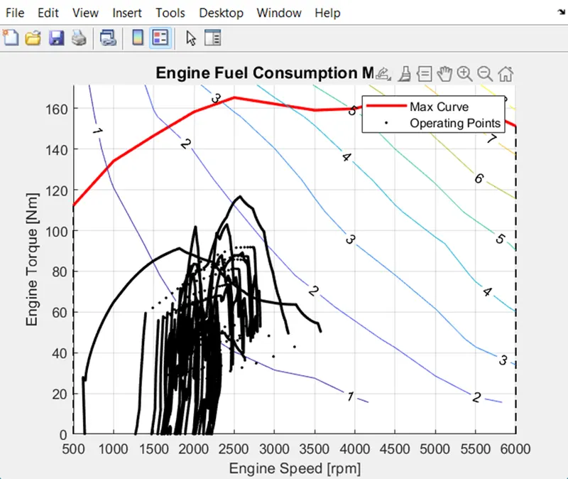Figure 8: Engine operating points for the HWFET cycle.

CONCLUSION:

Hence, we have studied how the Conventional Vehicle Model is designed and simulated by using MATLAB coding and Simulink. Also, I learned how to plot the graphs for different drive cycles.

Google Drive link: All Files