Project - Speed Control of a Direct Current (DC) motor

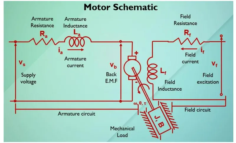
Schematically shown in the Figure

Theory-

What is a DC Motor?
--> A DC motor is defined as a class of electrical motors that convert electrical direct current electrical energy into mechanical energy.
From the above definition, we can conclude that any electric motor that is operated using direct current or DC is called a DC motor.
We will understand the DC motor construction and how a DC motor converts the supplied DC electrical energy into mechanical energy in the next few sections.

Parts of a DC Motor:-
1. Armature or Rotor:
The armature of a DC motor is a cylinder of magnetic laminations that are insulated from one another. The armature is perpendicular to the axis of the cylinder.
The armature is a rotating part that rotates on its axis and is separated from the field coil by an air gap.
2. Field Coil or Stator:
A DC motor field coil is a non-moving part on which winding is wound to produce a magnetic field.
This electro-magnet has a cylindrical cavity between its poles.
3. Commutator:
The commutator of a DC motor is a cylindrical structure that is made of copper segments stacked together but insulated from each other using mica.
The primary function of a commutator is to supply electrical current to the armature winding.
4. Brushes:
The brushes of a DC motor are made with graphite and carbon structure.
These brushes conduct electrical current from the external circuit to the rotating commutator.
Hence, we come to understand that the commutator and the brush unit are concerned with transmitting the power from the static electrical circuit to the mechanically rotating region or the rotor.

DC Motor Working:-
--> A magnetic field arises in the air gap when the field coil of the DC motor is energised. The created magnetic field is in the direction of the radii of the armature.
The magnetic field enters the armature from the North pole side of the field coil and exits the armature from the field coil's South pole side. The conductors located on the other pole are subjected to a force of the same intensity but in the opposite direction.
These two opposing forces create a torque that causes the motor armature to rotate.
Principle:
When kept in a magnetic field, a current-carrying conductor gains torque and develops a tendency to move. In short, when electric fields and magnetic fields interact, a mechanical force arises.
This is the principle on which the DC motors work.

What is a PID Controller?
--> A PID controller is an instrument used in industrial control applications to regulate temperature, flow, pressure, speed and other process variables.
PID controllers use a control loop feedback mechanism to control process variables and are the most accurate and stable controllers.
PID control is a well-established way of driving the system towards a target position or level.
It's practically ubiquitous as a means of controlling temperature and finds application in myriad chemical and scientific processes as well as automation.
PID control uses closed-loop control feedback to keep the actual output from a process as close to the target or setpoint output as possible.

• Here the Speed control of a DC motor is either done manually by the operator or by an automatic control device.
• This is different to speed regulation where the speed is trying to be maintained or regulated against the natural change in the speed (rate) due to a change in the load on the shaft.

• So the speed can be varied by changing the:

  1. The terminal voltage of the armature V,
  2. The external resistance in the armature circuit R_a,
  3. The flux per pole.

• So Terminal voltage and external resistance involve a change that affects the armature circuit while flux consists of a change in the magnetic field.

• Therefore, speed control of a DC motor can be classified into the:

  1. Armature Control Methods
  2. Field Control Methods

In this Project, we use the Armature control method for the speed control of the DC motor:


The mathematical modelling of DC motor is,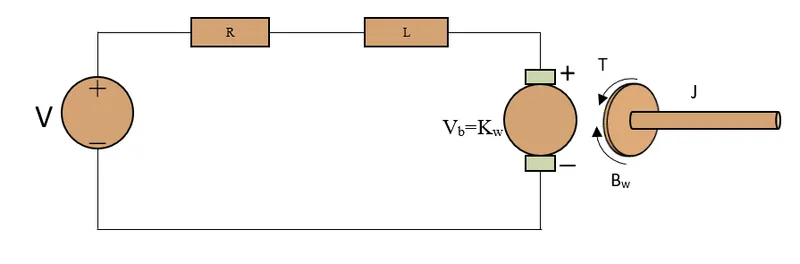

The DC motor Parameters are,

• J = Moment of Inertia of Rotor (kgm^2)
• B = Damping Constant (Nms)
• R = Ra = Armature resistance (ohm)
• L = La = Armature inductance (Henry)
• Vb = Back emf constant (volt)
• Kt = Motor Torque constant (Nm/Amp)
• V = Voltage (volt)

Motor torque, T = Kt*Ia, ...where Kt is torque constant and Ia is armature current

Back EMF, Vb = Kb*w, ...where Kb is back emf constant and w is the angular frequency in rad/sec

Equation finding steps ---

let Kt = Kb = K,

As per Kirchhoff"s closed loop law:-

La*(dIa/dt) + Ra*Ia = V - K*theta_dot -----------(1)

By Newton's second law we get:-

J*theta_dot_dot + B*theta_dot = K*Ia -----------(2)

where theta_dot = w (angular Velocity)

Transfer Function:-

By using the Laplace transform we get,

(La.s+Ra)Ia(s)= Vs(s)-K.s*theta(s) -----------(3)

Ia(s)= Vs(s)-k.s*theta(s) / (La.s+Ra)

s(J.s+B)*theta(s) = K*Ia(s) --------------(4)

w(s) = s.theta(s) = K*Ia(s) / J.s+B

The transfer function of the output angle, theta(s) is:-

theta_dot(s)/Vs(s) = K/[s(La.s+Ra)(J.s+B)+K^2]

The transfer function of angular velocity, w(s) is:-

w(s)/Vs(s) = K/[(La.s+Ra)(J.s+B)+K^2]

State-Space Equations for the DC Motor:-

(dIa/dt) = - R/L * I - 1/L * V - K/L*theta_dot

(dIa/dt) = - R/L * I - 1/L * V - K/L*w

(dw/dt) = - B/J*w + 1/J* K*Ia

Y(t)=w=theta_dot

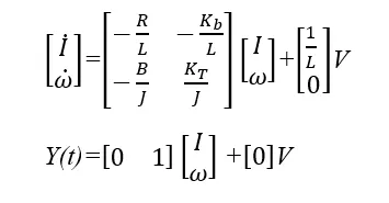
A state-space representation of the DC Motor:-

[dIa/dt ; dw/dt] = [ -R/L -Kb/L ; -B/J Kt/J ] [Ia ; w]+[1/L ; 0]*.V

Y(t) = [0 1] [Ia ; w]+[0]*.V

i.e,

MODEL:-

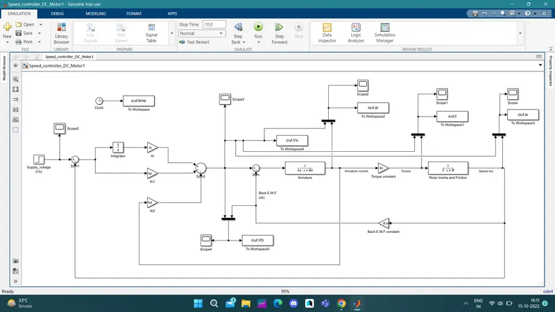
MATLAB SCRIPT CODE:-
% Parameters to design DC Motor Model

% Moment of Inertia of the rotor in kg-m^2
J = 0.01;

% Motor viscous friction constant in Nm-s
B= 0.1;

% Back E.M.F constant in v/rad/sec
Km= 0.01;

% Motor torque constant in Nm/amp
Kt=0.01;

% Resistance of the armature circuit in ohms
Ra= 1.0;

% Inductance of the armature circuit in henries
La= 0.5;

% Equivalent wn
fn= 1.0; % 1 Hz Natural frequency
wn= 2*pi*fn; % Natural frequency in rad/s

% Design parameters
zeta= 0.5; % For an Under-damped System

% jacobian matrices
A=[-B/J Kt/J; -Km/La -Ra/La];
C=[0 ; 1/La];

% Desired poles
p1= - zeta*wn + wn*sqrt(zeta^2 - 1);
p2= - zeta*wn - wn*sqrt(zeta^2 - 1);
P=[p1;p2];

% Pole placement design
K=place(A,C,P);
K(1)=38.3132;
K(2)=-2.8584;

% Kp and Kd gains obtained using the PLACE command
kp=K(1); % proportional gain
kd=K(2); % derivative gain
ki=0.01; % integrative gain assuming it to be 0.01

% Dynamics
% x1_dot = x2
% x2_dot = (-k/m)*x1 +(1/m)*u
% x2_dot = (-k/m)*x1 +(1/m)*[Kp*(x1ref-x1)+ki*integral(x1ref-x1)*dt-Kd*x2

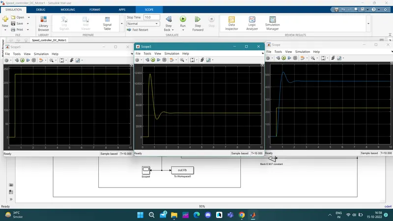
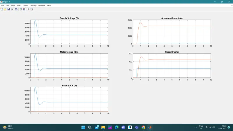
So we need to pick or alter the values of Kp, Kd, and Ki gains to meet the controlled objectives like settling time, overshoot, and steady-state error.
We increased & decreased the value of Ki & check the result to meet the controlled objectives:-For steady-state error reduction, the Ki value should change, we can perform a trial and error method here, changing the value of Ki to 10,

% Kp and Kd gains obtained using the PLACE command
kp=K(1); % proportional gain
kd=K(2); % derivative gain
ki=10; % integrative gain

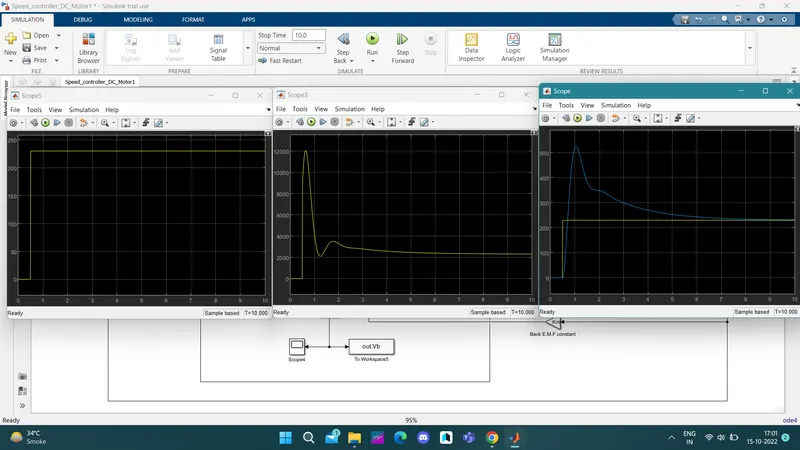
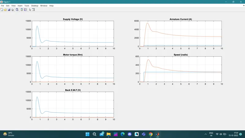
Compared with Ki = 10 value the steady-state error is reducing but not desired value, choosing ki=20,

% Kp and Kd gains obtained using the PLACE command
kp=K(1); % proportional gain
kd=K(2); % derivative gain
ki=20; % integrative gain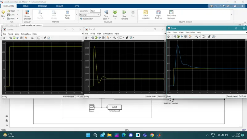

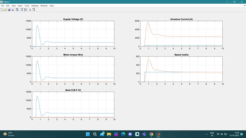
Compared with Ki = 20 value the steady-state error is reducing but not desired value, choosing ki=30,

% Kp and Kd gains obtained using the PLACE command
kp=K(1); % proportional gain
kd=K(2); % derivative gain
ki=30; % integrative gain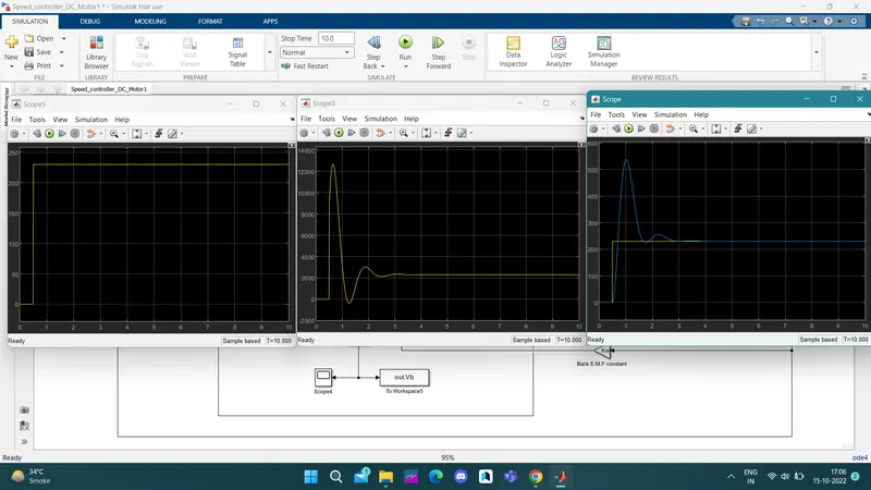

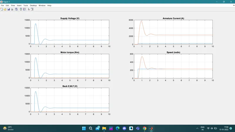
Compared with Ki = 30 value the steady-state error is reduced since we are almost near to the desired output, we can try changing the value to ki=40 and see the output if the actual output,

% Kp and Kd gains obtained using the PLACE command
kp=K(1); % proportional gain
kd=K(2); % derivative gain
ki=40; % integrative gain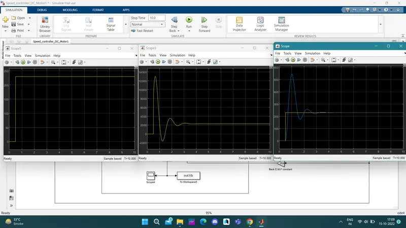

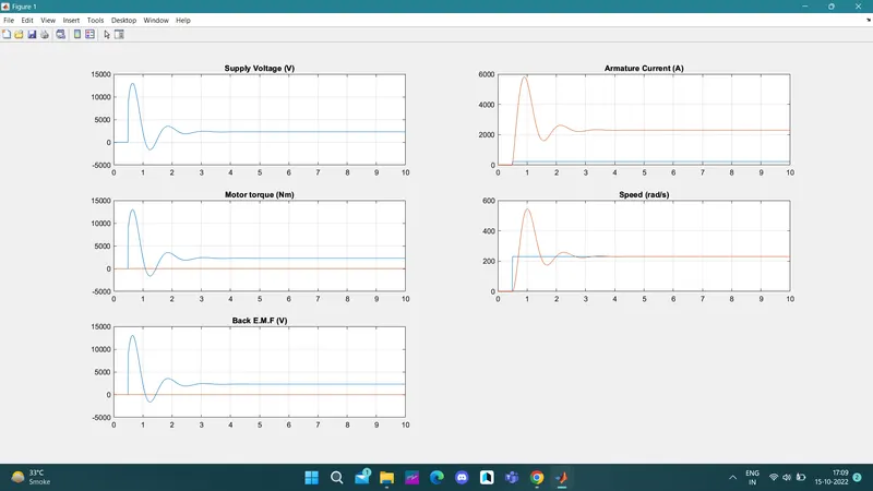
The actual output curve is wobbling near the desired output, trying to stabilize the curve, choosing ki=35,

% Kp and Kd gains obtained using the PLACE command
kp=K(1); % proportional gain
kd=K(2); % derivative gain
ki=35; % integrative gain

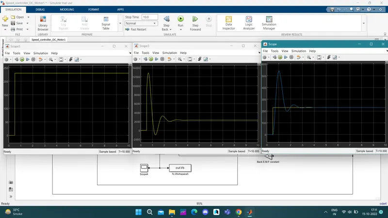
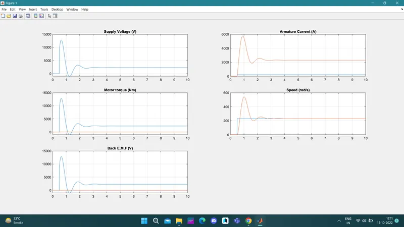
There is a reduction in the Steady-state error but there is a large overshoot in response, the Overshoot can be reduced by Kd gain, assuming kd=-1.5;

% Kp and Kd gains obtained using the PLACE command
kp=K(1); % proportional gain
kd=-1.5; % derivative gain
ki=35; % integrative gain

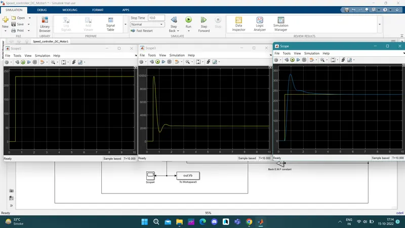
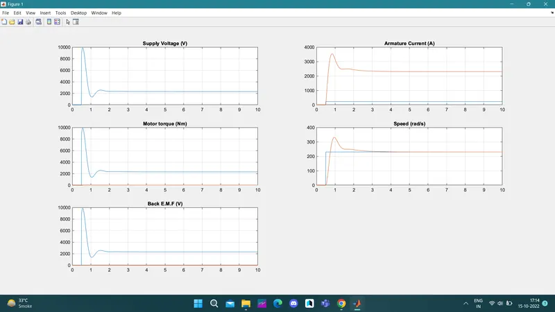
Compared to kd=-2.8584, There is a reduction in the overshoot but further, the overshoot can be reduced by Kd gain to get desired overshoot response, assuming kd=-0.5;

% Kp and Kd gains obtained using the PLACE command
kp=K(1); % proportional gain
kd=-0.5; % derivative gain
ki=35; % integrative gain

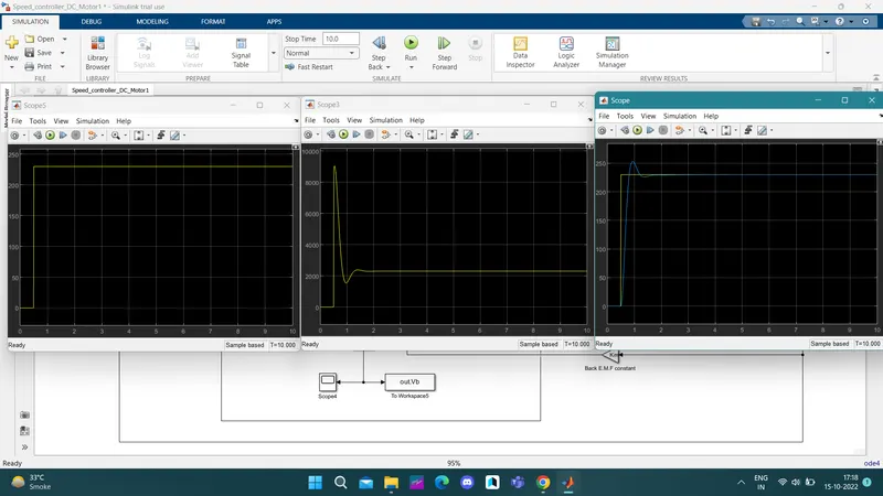
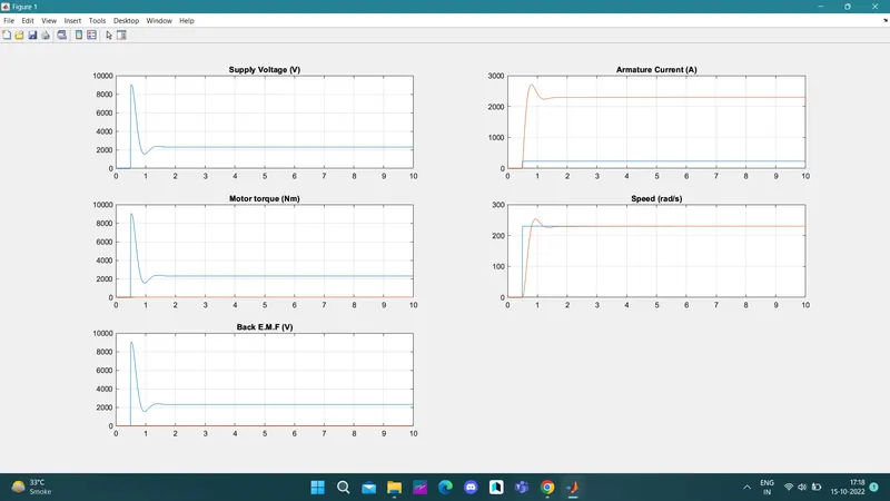
From the above values of Kd, Ki & Kp the most suitable values that give the best response are:-

% Kp and Kd gains obtained using the PLACE command
kp=38.3132; % proportional gain
kd=-0.5; % derivative gain
ki=35; % integrative gain

Summary -

• A Direct Current (DC) Machine can function as a generator or motor.
• A Direct Current (DC) Machine consists of a rotor (rotating part) with an armature winding providing the electrical circuit and a stator (stationary part) with field winding serving as a magnet when energized.
• While operating in generator mode, a prime mover is coupled to the rotor, allowing it to rotate in the magnetic field which induces
• Electromotive Force (EMF) in the conductors mounted on the rotors.
• While operating in motor mode, the electrical energy supplied to the armature winding and the field winding contributes to a rotating magnetic field that forces the rotor to rotate which as result generates mechanical torque.
• A PID controller design is demonstrated to obtain the desired angular speed using the appropriate supply voltage. i.e., We can control the speed of a DC Motor using a Proportional, Integral and Derivative (PID) control design.
• Designed and successfully tested a controller to maintain the desired speed for the motor.

Conclusion -

1. This week we learnt, the modelling of a Direct Current (DC) Generator and Motor.
2. And also we learnt about the application of the PID control design techniques for the speed control of a DC Motor.
3. p1 = -3.1416 + 5.4414i and p2 = -3.1416 - 5.4414i
   Poles lie on the left-hand side of the S-plane, this indicates the system is stable.
4. The PID controller block manages the control objectives i.e. Settling time < 2 sec, Overshoot < 5 % and Steady-state error < 1 %.
5. Designed a Proportional, Integral and Derivative (PID) control and successfully tested the controller to maintain the desired speed for the motor.