Week 7 State of charge estimation

OBJECTIVE

Download a file from matlab file exchange and do the following and explain the following

a.Simulate the 3 test cases from harness dashboard and write a detailed report on the results.

b.What is coulomb counting? Refer to the downloaded model and explain how BMS implements coulomb counting for SOC estimation

PROCEDURE

The following BMS Simulink files to be opened before running the simulation

BMS Closed loop

It consists of BMS software and Battery plant subsystem which can be opened as a seperate file.

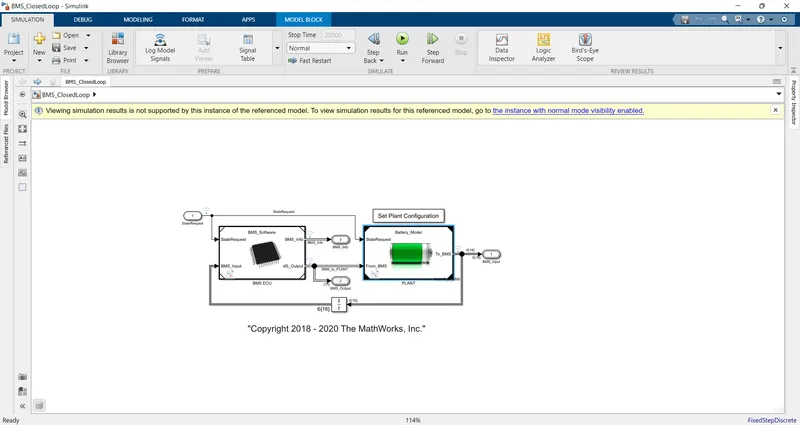
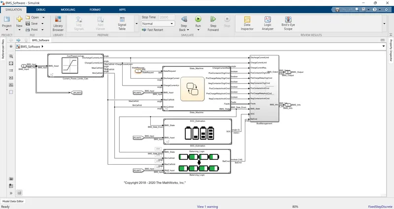
Now, open BMS software in seperate window. It can be opened as BMS ECU

In BMS ECU, it calculates the result that we need, which is SOC,Battery balancing, Battery state, Battery Voltage, Current drawn,Thermal range.

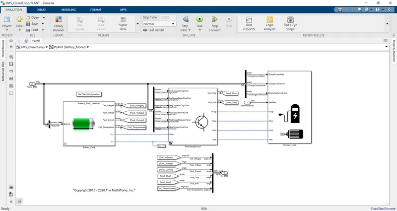
Now, we are taking a look inside battery plant model.

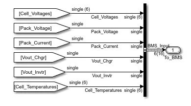
From plant model, BMS receives 6 parameters which are shown below

The BMS Closed loop is under BMS_Closedloop_Harness_Dashboard where we send one of the 3 state request to the BMS closed loop and then BMS displays the simulation result.

The figure below shows BMS_Closedloop_Harness_Dashboard

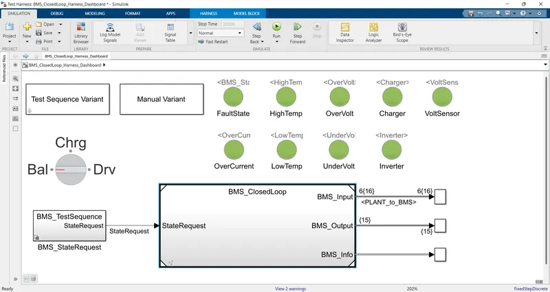
We are giving 3 cases by double clicking on Test Sequence Variant Subsystem

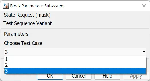
After selecting either 1,2,3 we can Simulate and see the result.

1.Simulate the 3 test cases from harness dashboard and write a detailed report on the results

EXPLANATION OF THE RESULT

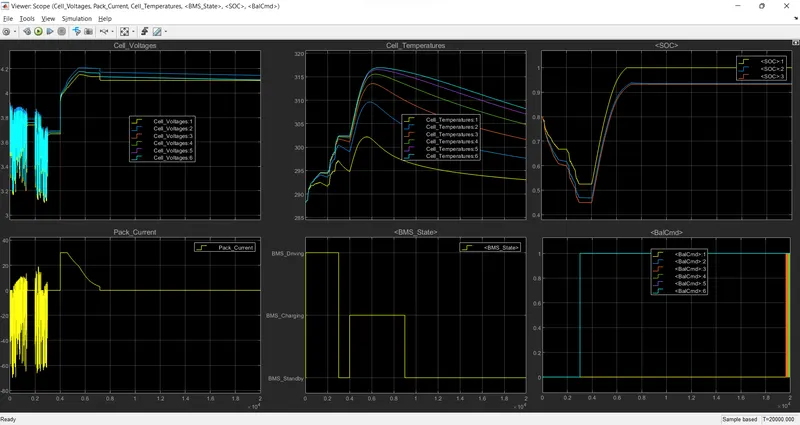
1) Selecting 1 on Test Sequence Variant Subsystem and simulate. The result can be shown below

a) Cell Voltage and Pack current

Initially during driving cycle upto 3000 sec, all the 6 cell voltage varies between 3.9 V and 3.18 V. When the cells getting discharged, the voltage comes down and then again charged due to regenerative braking. So, all the 6 battery signals oscilated between 3.9 V to 3.18 V. The pack current value is also oscilated wrt the cell voltage.

From 3000-4000 sec, the vehicle comes to standby state. In this condition, battery is not getting discharged. So, the voltage remains steady. The pack current is also not varying during this period.

From 4000-9000 sec, the charging happens. From 4000-5000 sec, the constant current charging happening which can be understood from flattening graph of the current circuit. The supply current is around 30 A. While charging the cell voltage increases. After 5000 sec, the constant Voltage charing happens. During this time, the pack current is reduced to zero. During the end of charging the bms comes to standby state. During this time, the cell balancing happens. If we look at the voltage graph at the end of the simulation, all the cell voltage comes to converge each other, ie all the cells try to balance the voltage. The cell balancing can be analysed using the figure later on.

b) Cell Temperatures

Here, all the 6 cells are connected together. One side of cell 6 is thermally insulated and other side is connected to cell 5. Then all other cells are connected in series together sharing common thermal boundary. But for the last cell(cell 1), one side is connected to cell 2 and other side is open to atmosphere.

During the entire simulation time, the thermal range of all the cells varying similarly. The cell 1 is operating lower temperature because one end is open to atmosphere, so it have lower temperature than other cells. The cell temperature is increasing if we move from cell 1 to cell 6. Cell 6 have higher temperature,because its one end is thermally insulated.

c) SOC

The SOC graph shows 3 types of SOC estimation. The yellow line indicates Columb Counting method, the second blue and red line indicated UKF and EKF method which estimates SOC more accurately than Columb Counting

d) BalCmd

This graph shows the cell balancing

Similar to some voltage difference in Voltage graph, cell balancing also behaves like that.

The cell 1,3,4,6 try to balance each other.

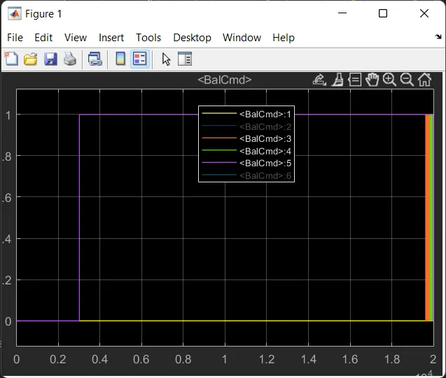
This can be understood by zooming the vertical lines during the end of simulation.

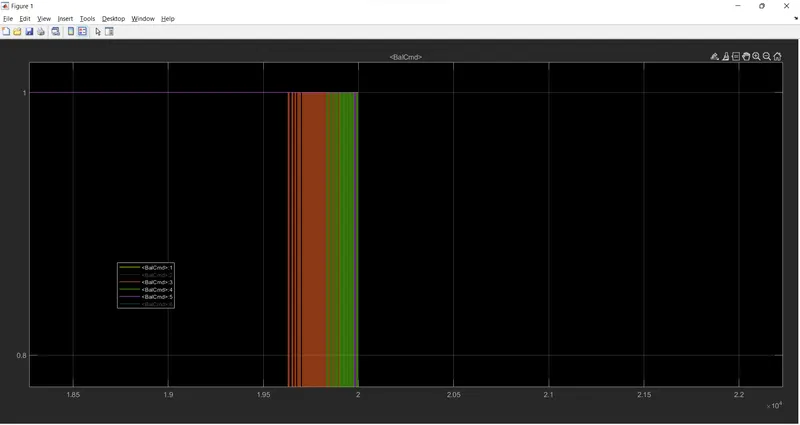
But cell 2 and cell 6 not balancing with cell 1 as shown below

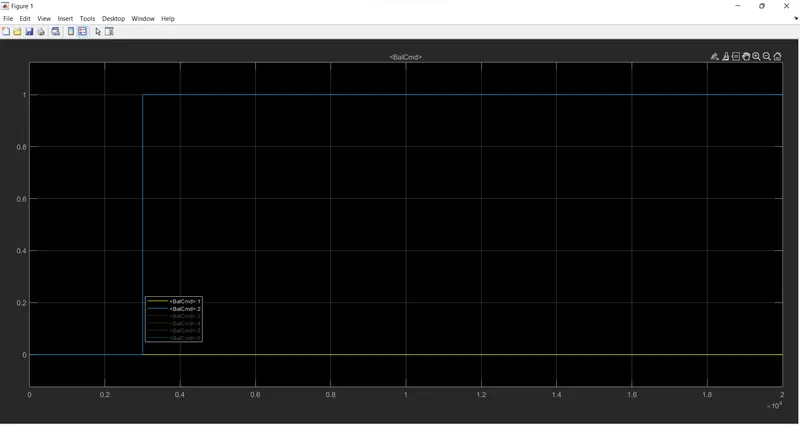
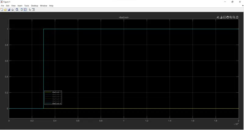
But cell 1,3,4,6 are in perfect balancing.

2) Selecting 2 on Test Sequence Variant Subsystem and simulate. The result can be shown below

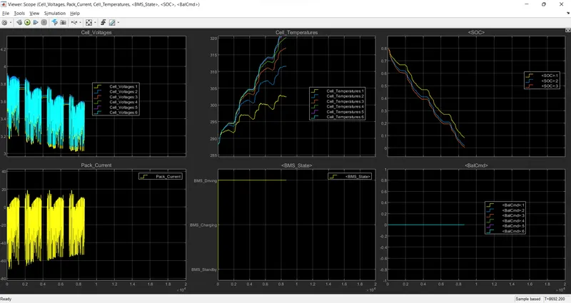
This is the case of driving cycle only. When the cell voltage comes down or when the cell temperature rises the vehicle stops and it is a faulty state. The SOC comes down to zero at this point. In this case cell balancing not happening

The cell voltage is coming down due to driving and the current consumption is gradually increases and stops during faulty state.

3) Selecting 3 on Test Sequence Variant Subsystem and simulate. The result can be shown below

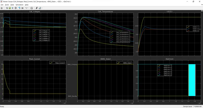
This is the case of charging only.

The charging starts from SOC=0.8.

While charging, the voltage of each cell suddenly increases. If we look at voltage graph, the cell 2 have higher voltage and other cells are coming to balanced stage during the end of the simulation. Cell 2 not getting balanced with other cell during charging. this can be understood if we look at cell voltage graph and BalCmd graph, as there is small gap between voltages of cell 2 with other cell. Also, the cell 2 at the end of simulation stage is at 1 in BalCmd while all other cells are at 0. the balancing process happens between 16000-18000 sec, which is shown as vertical lines in the graph.

The SOC suddenly increases during charging and it saturates during charging cycle. The same is the case of Cell Voltage during charging. The SOC is estimated using 3 methods are plotted in graph which is same as that of case 1.

The pack current comes to zero and saturates during charging.

The cell temperature of all cells suddenly rises, with each cell having different higher temperature same as explained for case 1. The cell temperature graph of all cells varies similarly. The detailed explanation is same as that of case 1.

During the end of simulation, the cell temperature reduces.

2.What is coulomb counting? Refer to the above model and explain how BMS implements coulomb counting for SOC estimation ?

The Coulomb counting method measures the discharging current of a battery and integrates the discharging current over time in order to estimate SOC . Coulomb counting method is done to estimate the, which is estimated from the discharging current, and previously estimated SOC values, . SOC is calculated by the following equation:

where:

• SoC(t) = estimated State of Charge at time, t
• SoC(t-1) = previous State of Charge at time t-1
• I(t) = charging or discharging current at time, t
• Q_n = battery cell capacity
• Δt = time step between t-1 and t

But there are several factors that affect the accuracy of Coulomb counting method including temperature, battery history, discharge current, and cycle life.

The SOC methods in this model can be find out by opening BMS Software. Inside it, open SOC_Estimation subsystem

After opening SOC_Estimation subsystem, we can find Columb Counting subsystem and EKF,UKF subsystem

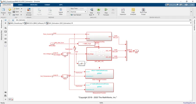
Columb counting receives Current measurement and Temperature measurement as input from battery Measurement Function. The Coulomb Counting subsystem is shown below

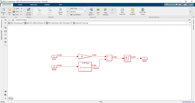
The input current is then passed through gain to reduce its value to 1/3600, so as to get capacity in Ah. The temperature signals is passed through 1-D look up table to get corresponding values of capacity. Then both the capacity is divided and then passed to Discrete-Time Integrator to get SOC value.