Week 4.1 - Genetic Algorithm
To find the global maxima of a function,I m taking the negative of a function and find it's global minima using GA in matlab.Then multiplying the result(global minima) by -1 gives the global maxima of a function.
The negative function name is stgcpymax.m
This is exactly just like taking the mirror image of a function(Reference video of NPTEL IIT Guwahati,Prakash Kotecha https://www.youtube.com/watch?v=aJKuM4U-eYg&t=3715s )
The function to find the global maxima is stgcpy2.m. This is only a code.I didn't done application in main code.But I found error if I use it,which will be explained later
function [Fmin]= stgcpy2(vec)
vec1=vec(1);vec2=vec(2);
fx1=(sin(5.1*pi.*vec1+0.5))^6;
fx2=exp(-4*log(2)*((vec1-0.0667)^2)/0.64);

fy1=(sin(5.1*pi.*vec2+0.5))^6;
fy2=exp(-4*log(2)*((vec2-0.0667)^2)/0.64);


Fmin=fx1.*fx2.*fy1.*fy2;

end
The main program for the challenge shown below
clear all,close all,clc;
%Making the interval of domain x and y as (-1,1) because there is no local
%or global extrema outside this domain.We understand it by plotting it
x=linspace(-1,1,150);
y=linspace(-1,1,150);

[xx yy]=meshgrid(x,y);
% Storing the values of 150 X 150 matrix for the stalagmite function in
% variable F
for i=1:length(xx)
    for j=1:length(yy)
        inp_vec(1)=xx(i,j);
        inp_vec(2)=yy(i,j);
        F(i,j)=stgcpymax(inp_vec);
    end
end


%Study 1
%Getting optimum values from GA by evaluating stalagmite function for 50
%times.In this case,GA doesn't know the search space for local and
%global extrema
tic
for i=1:50
[input1,fopt1(i)]=ga(@stgcpymax,2);
xopt1(i)=input1(1);                  %xopt1 & yopt1 are the values of x and y at which the function has minimum value

yopt1(i)=input1(2);
                                     %Taking the negative of xopt1,yopt1 &
                                     %fopt1 in order to find optimum values
                                     %of global maxima
xopt1_gmax(i)=-xopt1(i);yopt1_gmax(i)=-yopt1(i);
fopt1_gmax(i)=-fopt1(i);


end
study_time1=toc;
figure(1)
subplot(2,1,1)
hold on
surfc(-x,-y,-F)
shading interp
plot3(xopt1_gmax,yopt1_gmax,fopt1_gmax,'marker','o','markerfacecolor','r')
xlabel('x axis');ylabel('y axis');
legend('','','GA Evaluation');
title('Stalagmite Function Curve & GA Evaluation of optima');
subplot(2,1,2)
plot(fopt1_gmax)
xlabel('Iterations');ylabel('Optimum function values');zlabel('Stalagmite Function');

%Study 2
%Diffrenence from Study 1 is that we define search space for x and y such
%that GA function will search for extremas within that range only
tic
for i=1:50
[input2,fopt2(i)]=ga(@stgcpymax,2,[],[],[],[],[-1;-1],[1;1]);
xopt2(i)=input2(1);yopt2(i)=input2(2);
xopt2_gmax(i)=-xopt2(i);yopt2_gmax(i)=-yopt2(i);
fopt2_gmax(i)=-fopt2(i);

end
study_time2=toc;
figure(2)
subplot(2,1,1)
hold on
surfc(-x,-y,-F)
shading interp
plot3(xopt2_gmax,yopt2_gmax,fopt2_gmax,'marker','o','markerfacecolor','r')
title('Stalagmite Function Curve & GA Evaluation of optima');
xlabel('x axis');ylabel('y axis');zlabel('Stalagmite Function');
legend('','','GA Evaluation');
subplot(2,1,2)
plot(fopt2_gmax)
xlabel('Iterations');ylabel('Optimum function values');


%Study 3
%Changing the population size to 500 so as to converge the solution to global extrema such
%that it get approximate same values of extremas at every time during
%execution of program
options=optimoptions('ga','PopulationSize',500);
tic
for i=1:50
[input3,fopt3(i)]=ga(@stgcpymax,2,[],[],[],[],[-1;-1],[1;1],[],options)
xopt3(i)=input3(1);yopt3(i)=input3(2);

xopt3_gmax(i)=-xopt3(i);yopt3_gmax(i)=-yopt3(i);

fopt3_gmax(i)=-fopt3(i);
end
study_time3=toc;
figure(3)
subplot(2,1,1)
hold on
surfc(-x,-y,-F)
shading interp
plot3(xopt3_gmax,yopt3_gmax,fopt3_gmax,'marker','o','markerfacecolor','r');
legend('','','GA Evaluation');
xlabel('x axis');ylabel('y axis');zlabel('Stalagmite Function');
title('Stalagmite Function Curve & GA Evaluation of optima');
subplot(2,1,2)
plot(fopt3_gmax)
xlabel('Iterations');ylabel('Optimum function values');
Stalagmite Function 1:stgcpy2.m (Main function to find global maxima)
function [Fmin]= stgcpy2(vec)
vec1=vec(1);vec2=vec(2);
fx1=(sin(5.1*pi.*vec1+0.5))^6;
fx2=exp(-4*log(2)*((vec1-0.0667)^2)/0.64);

fy1=(sin(5.1*pi.*vec2+0.5))^6;
fy2=exp(-4*log(2)*((vec2-0.0667)^2)/0.64);


Fmin=fx1.*fx2.*fy1.*fy2;

end
Stalagmite Function 2:The negative of stgcpy.m which is stgcpymax.m
function [F]= stgcpymax(vec)
vec1=vec(1);vec2=vec(2);
fx1=(sin(5.1*pi.*vec1+0.5))^6;
fx2=exp(-4*log(2)*((vec1-0.0667)^2)/0.64);

fy1=(sin(5.1*pi.*vec2+0.5))^6;
fy2=exp(-4*log(2)*((vec2-0.0667)^2)/0.64);


F=-fx1.*fx2.*fy1.*fy2;


end
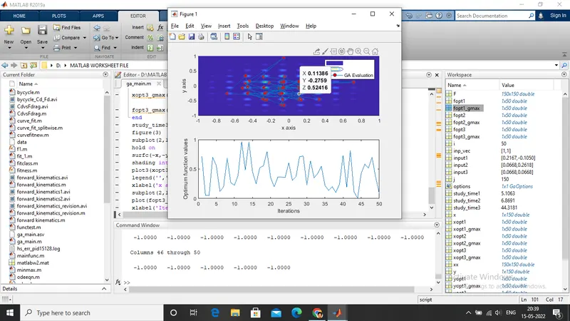
OUTPUT Study 1
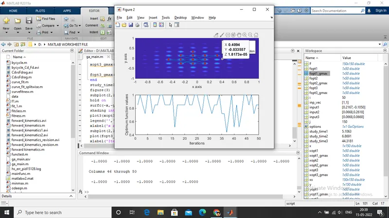
OUTPUT STUDY 2
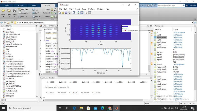
OUTPUT STUDY 3
EXPLANATION OF OUTPUT & CODE
The red dots shown in the plots converges to one peak point in OUTPUT 3(Study 3) as the population size is increased.This is the property of GA.Thus,we get accurate values of global maxima every time the code runs and we use iterations for this purpose
By default,GA takes population size as 50.This is the case for Study 2 or OUTPUT 2.We are modifying the population size to 500 in Study 3,so that the solution converges to global maxima.In Study 2, GA cannot find the perfect result as the population size is not enough.So, the solution(population) of GA is approaching the local maximas and global maximas.
By increasing the population size, higher probability of finding fitted parents for the function and find the optimal solution.
For Study 2 & 3, I defined lower and upper bound as [-1;-1] & [1;1],such that GA evaluation should not go outside this range so as to find the optimal solution.
The domain of the function also I mentioned as [-1;-1] & [1;1] & GA search space I mentioned in this region.
For Study 1(OUTPUT 1),there is no upper and lower bound. So GA can search anywhere to find the optimal solution.
ERROR IN CODE
The variable hhh is used to end the operation upto study 2 for saving time.It's not an error
clear all,close all,clc;
%Making the interval of domain x and y as (-1,1) because there is no local
%or global extrema outside this domain.We understand it by plotting it
x=linspace(-1,1,150);
y=linspace(-1,1,150);

[xx yy]=meshgrid(x,y);
% Storing the values of 150 X 150 matrix for the stalagmite function in
% variable F
for i=1:length(xx)
    for j=1:length(yy)
        inp_vec(1)=xx(i,j);
        inp_vec(2)=yy(i,j);
        F(i,j)=stgcpy2(inp_vec);
    end
end


%Study 1
%Getting optimum values from GA by evaluating stalagmite function for 50
%times.In this case,GA doesn't know the search space for local and
%global extrema
tic
for i=1:50
[input1,fopt1(i)]=ga(@stgcpymax,2);
xopt1(i)=input1(1);                  %xopt1 & yopt1 are the values of x and y at which the function has minimum value

yopt1(i)=input1(2);
                                     %Taking the negative of xopt1,yopt1 &
                                     %fopt1 in order to find optimum values
                                     %of global maxima
xopt1_gmax(i)=-xopt1(i);yopt1_gmax(i)=-yopt1(i);
fopt1_gmax(i)=-fopt1(i);


end
study_time1=toc;
figure(1)
subplot(2,1,1)
hold on
surfc(x,y,F)
shading interp
plot3(xopt1_gmax,yopt1_gmax,fopt1_gmax,'marker','o','markerfacecolor','r')
xlabel('x axis');ylabel('y axis');
legend('','','GA Evaluation');
title('Stalagmite Function Curve & GA Evaluation of optima');
subplot(2,1,2)
plot(fopt1_gmax)
xlabel('Iterations');ylabel('Optimum function values');zlabel('Stalagmite Function');

%Study 2
%Diffrenence from Study 1 is that we define search space for x and y such
%that GA function will search for extremas within that range only
tic
for i=1:50
[input2,fopt2(i)]=ga(@stgcpymax,2,[],[],[],[],[-1;-1],[1;1]);
xopt2(i)=input2(1);yopt2(i)=input2(2);
xopt2_gmax(i)=-xopt2(i);yopt2_gmax(i)=-yopt2(i);
fopt2_gmax(i)=-fopt2(i);

end
study_time2=toc;
figure(2)
subplot(2,1,1)
hold on
surfc(x,y,F)
shading interp
plot3(xopt2_gmax,yopt2_gmax,fopt2_gmax,'marker','o','markerfacecolor','r')
title('Stalagmite Function Curve & GA Evaluation of optima');
xlabel('x axis');ylabel('y axis');zlabel('Stalagmite Function');
legend('','','GA Evaluation');
subplot(2,1,2)
plot(fopt2_gmax)
xlabel('Iterations');ylabel('Optimum function values');

hhh
%Study 3
%Changing the population size to 500 so as to converge the solution to global extrema such
%that it get approximate same values of extremas at every time during
%execution of program
options=optimoptions('ga','PopulationSize',500);
tic
for i=1:50
[input3,fopt3(i)]=ga(@stgcpymax,2,[],[],[],[],[-1;-1],[1;1],[],options)
xopt3(i)=input3(1);yopt3(i)=input3(2);

xopt3_gmax(i)=-xopt3(i);yopt3_gmax(i)=-yopt3(i);

fopt3_gmax(i)=-fopt3(i);
end
study_time3=toc;
figure(3)
subplot(2,1,1)
hold on
surfc(-x,-y,-F)
shading interp
plot3(xopt3_gmax,yopt3_gmax,fopt3_gmax,'marker','o','markerfacecolor','r');
legend('','','GA Evaluation');
xlabel('x axis');ylabel('y axis');zlabel('Stalagmite Function');
title('Stalagmite Function Curve & GA Evaluation of optima');
subplot(2,1,2)
plot(fopt3_gmax)
xlabel('Iterations');ylabel('Optimum function values');
For Study 1 & Study 2,I plot using surf(x,y,F) instead of surf(-x,-y-,-F). I define F=stgcpy2(vec) instead of F=stgcpymax(vec). When GA evaluates this, the red colour point doesn't come exactly over local or global optima.
The error output is shown below
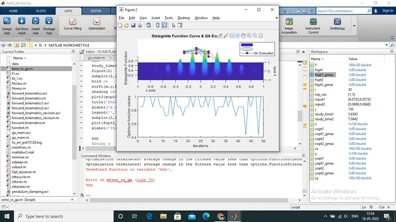
So, I put -x,-y,-F in surf done the GA evaluation
SYNTAX AND EXPLANATION OF GA
[input,fopt]=ga(@stalagmite,nvars,[],[],[],[],[LB],[UB],[],[],options)
input is the value at which GA predicts most optimum values fopt;
@stalagmite is the function name for which the GA evaluates global optimas(minima);
nvars is the number of variables in function. In our program, it's only 2,which is vec1 & vec2;
The next four square brackets [],[],[],[] corresponds to coefficients of linear inequalities and linear equalities constraints respectively. The first 2 [],[] is for linear inequalities and next 2 [],[] is for linear equalities.The constraints is to represents the feasible region for GA search space
[LB],[UB] represents the lower bounds and upper bounds for search space of GA;
The next [] represents the function for non linear inequality constraints;
The next [] represents the integer constraints. If there is integer constraints, the non-linear inequality constraint should be null;
The next options represents that we are editing the default values for better results.In our challenge,we are changing the population size to 500.The default values is 50 for five or few variables
GA Explanation
The GA uses the concept of selecting 2 random parents,then produce children by cross over or mutation and continue this to next generation as iteration(in optimization tool box app in matlab) until we find the most fitted values of function as optimum solution. Sometimes, the iteration is terminated based on stopping criteria.
If GA select an Elite parent from population size, the chance to get the optimum values is very high