Week 3 - Solving second order ODEs

PROGRAM FOR ODE EQUATION SOLUTION AND OSCILATION OF SIMPLE PENDULUM

clear all;close all;clc;

b=0.05;                             %damping coefficient
g=9.81;                             %gravity in m/s2
l=1;                                %length of the pendulum in m
m=1;                                %mass of the ball in kg
theta_0=[0;3];                      %Angular displacement=0 rad,Angular velocity=3 rad/sec at t=0
t_span = linspace(0,20,100);        %Time period defined for oscilation between 0-20 sec
%Solving first order ODE using ode45.The variables are theta and t
%[t]=[100 equal time interval between 0 to 20]
%[result]=Obtaining 100 values for displacement and velocity as 100X2 matrix]
[t,result]=ode45(@(t,theta) odesol(t,theta,b,g,l,m),t_span,theta_0)
%Plotting the values of t and result
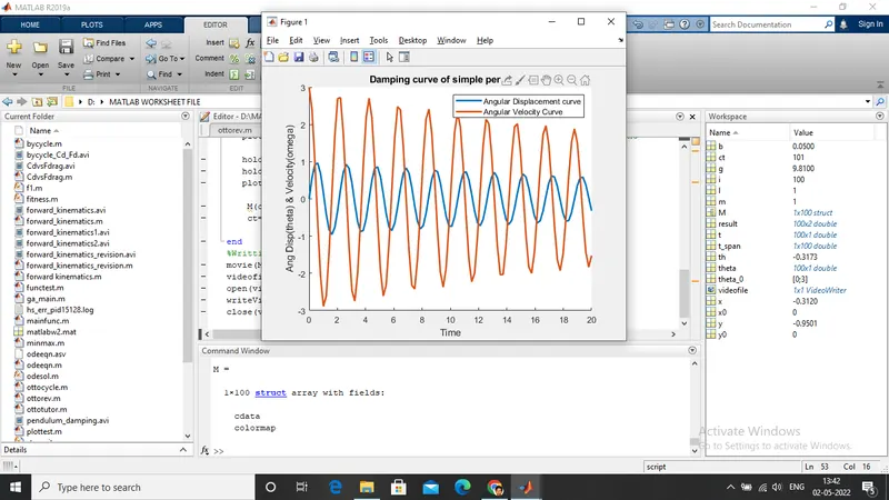
figure(1)
hold on
plot(t,result,'linewidth',2)
xlabel('Time');ylabel('Ang Disp(theta) & Velocity(omega)');
legend('Angular Displacement curve','Angular Velocity Curve');
title('Damping curve of simple pendulum');

%ANIMATION as a part of challenge

x0=0;y0=0;                      %Initialising (0,0) as cordinate for fixed end of pendulum
ct=1;
for i=1:length(result(:,1))
    theta=result(:,1);      %Accessing the values of first column of matrix [result]
    th=theta(i);            %Storing the values of [result] as per iteration
    %x and y explained in pdf attached
    x=l*sin(th);
    y=-l*cos(th);
    
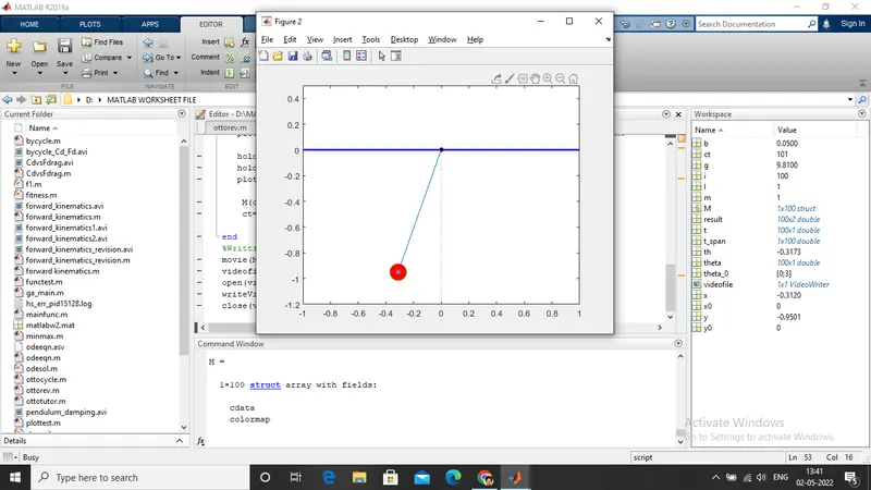
    figure(2)
    hold off
    plot([x0 x],[y0 y])                             %Plotting string of pendulum
    axis([-1 1, -1.2 0.5])                          %Shifting axes to look better
   hold on
   plot([0 0],[0 -1.2],':')                                     %Reference line about which pendulum oscilates
   plot([-1 1],[0 0],'linewidth',2,'color','b')                 %Rod at fixed end
   plot(x0,y0,'O','markersize',5,'markerfacecolor','black')     %Fixed end point
   plot(x,y,'O','markersize',20,'markerfacecolor','r')          %Free end point
    
   hold off
   hold on
   plot(x,y,'*')                    %Marking * at centre point of O
      
    M(ct)=getframe(gcf)             %Getting movie frame
    ct=ct+1;                        %Incrementing counter for movie frame
    
end
%Writting movie file
movie(M)
videofile=VideoWriter('pendulum_damping.avi','Uncompressed AVI');
open(videofile)
writeVideo(videofile,M)
close(videofile)

ODE SOLUTION FUNCTION

function [dtheta_dt]= odesol(t,theta,b,g,l,m)
theta1=theta(1);        %Storing the matrix index value(1) of theta in theta 1
theta2=theta(2);        %Storing the matrix index value(2) of theta in theta 2
dtheta1_dt=theta2;
dtheta2_dt=-(b/m)*theta2-(g/l)*sin(theta1);
dtheta_dt=[dtheta1_dt;dtheta2_dt];

end

OUTPUT Figure(1)

Graphical representation of damping of simple pendulum wrt time

OUTPUT Figure(2)

Oscilation of simple pendulum

EXPLANATION OF THE CODE IS SHOWN IN THE ATTACHED PDF.Filename is PENDULUM.PDF

YouTube link of animation is https://youtu.be/FMdg_ALB3nQ

OUTPUT VIDEO UPLOADED BELOW