Week 7 State of charge estimation

STATE OF CHARGE ESTIMATION

Objective:-

1. To stimulate the 3 test cases from harness dashboard and to write a detailed report on the results

2.What is coulomb counting? For the above model, to explain how BMS implements coulomb counting for SOC estimation.

Description:-

Objective 1:-

To download and open the closed loop BMS harness model:-

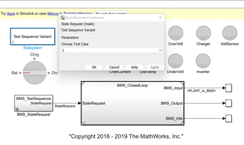
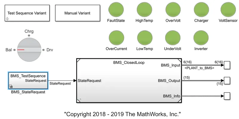
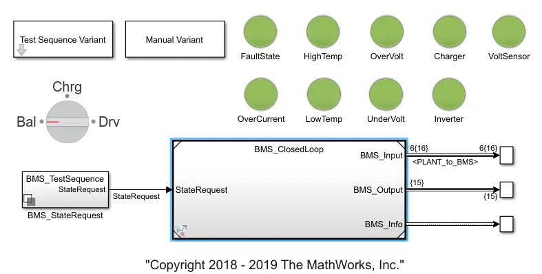
When you open the model in the Matlab, we can see the following dashboard:-

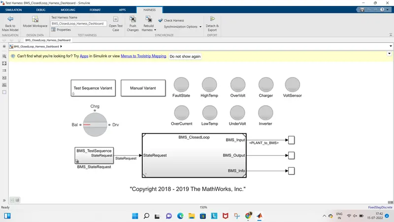
i)Test sequence variant block:-

This block is used to choose the different variant of test which we are going to implement.

ii)BMS Test sequence state request:-

It is an subsystem to provide the state request commanda

iii)BMS Closed loop:-

This is the main block of the model. When we double click this model and opened, it consists of two subsystems (a) BMS ECU & (b) PLANT, which is a battery unit.

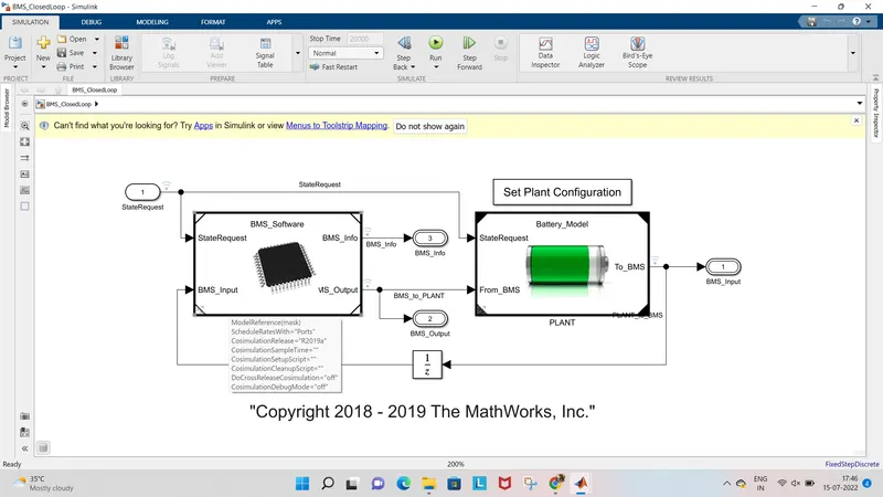
We can discuss the two main blocks seperately.

First let us discuss the Plant configuration block. When you double click the plant cinfiguration block, the following blocks will appear.

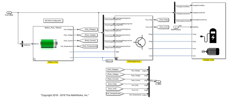
As we see in the above diagram, the Plant block consists of three seperate units consists of 1) Charger Load 2) Precharge circuit 3) The battery pack

a) Charger Load:-

The charger load block consists of a charger and motor which is responsible for the charging and discharging conditions of the battery pack. When you open the charger load block, the following sub system will get opened:-

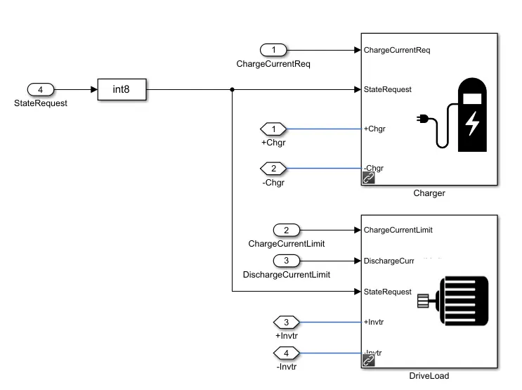
As we discussed above, it consists a Charger block, which is used for the charging conditions and a Motor load whuch is used for the discharge conditions. And as we can see that the charger is connected to the charger and motor is connected to the inverter since most of the Ev's used 3 phase induction motors, its important to convert the source. And when we again open the drive load block and charger block, the following blocks will aappear.

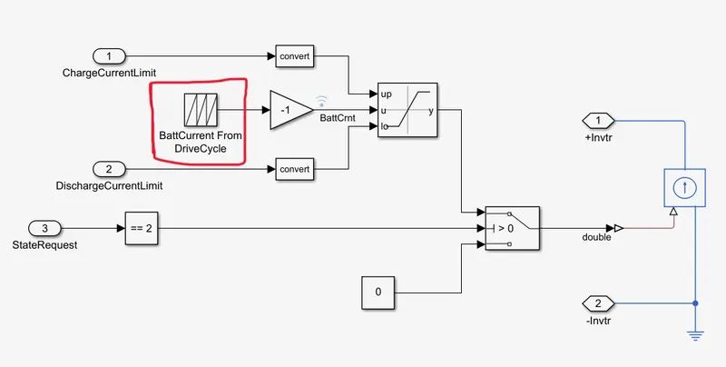
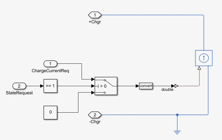
we can easily see that the motor is connected to the Drive cycle load, which provides alternationg values to the motor and hence the current, voltage and SOC can be analysed, since it is connected to the current source. Similarly the charger is also connected to the current source but in the opposite direction to the charger cuurrrent.

b) Precharger Circuit:-

Now let us see the detailed construction of the precharger circuit. When you double click and opens the pre charger block, the following subsystem will occur:-

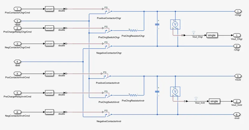
Basically, the precharge circuit is connected with pre charge resistors which are connected to the invertor as well as the charger. The switch blocks are used to connect and disconnect the precharge resistor to the entire block.

c)The battery pack circuit:-

When you double cllick and open the battery pack block, the following block will get open which consists of 2 systems in it.

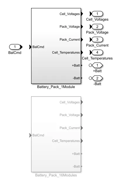
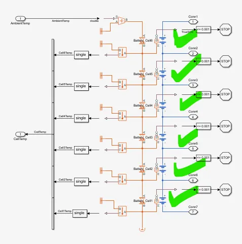
Here the 1st module consists of 6 cells in series and the 2nd unit consists of 6 modules in which each module contains 16 cells in series so that it comprises of 96 cells in series totally. When you open the single module block, you can see the six cells which are connected in series. And when you open the 16 module battery pack, these six cell series are connected to about 16 times which comprises a 96 series cell battery pack as follows. And also each of the cells are connected to the thermal management block, in which the temperatures can also be maintained.

Now we will move on to the BMS Software part:-

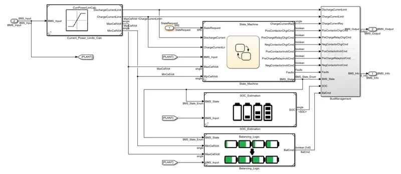
This segment is loke the heart block, since all the major characteristics of the battery are decided here. The Balancing, SOC estimation and all the inputs depends on the battery pack plant will get connected to this circuit and it gives the responses to all the input signals recieved. And hence all the battery functionalities can be decided with the help of this BMS part. These are the functions and importance of both the BMS and the plant configuration blocks. Now let us move into the problem statements:-

TEST 1:-

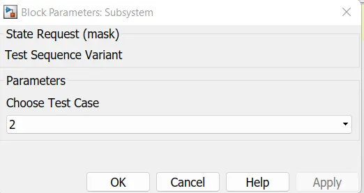
Now in the dashbooard, from the test sequence variant block, choose the test sequence as 1.

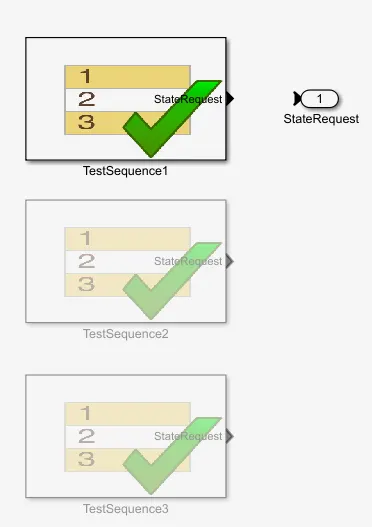
And that particular sequence is chosen by the 'BMS test sequence' block and the inputs are fed into the BMS closed loop circuit.

For the first sequence of test, the following conditions are provided:-

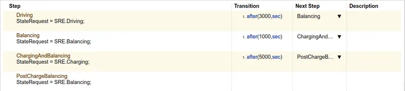
ie., Driving for 3000 seconds and then balancing willl happen for next 1000 seconds and then charging and balancing will be mutually done for the next 5000 seconds. Now when we analyse these conditions with the help of the scope, the following outputs will occur:-

OUTPUT FOR TEST CASE 1:-

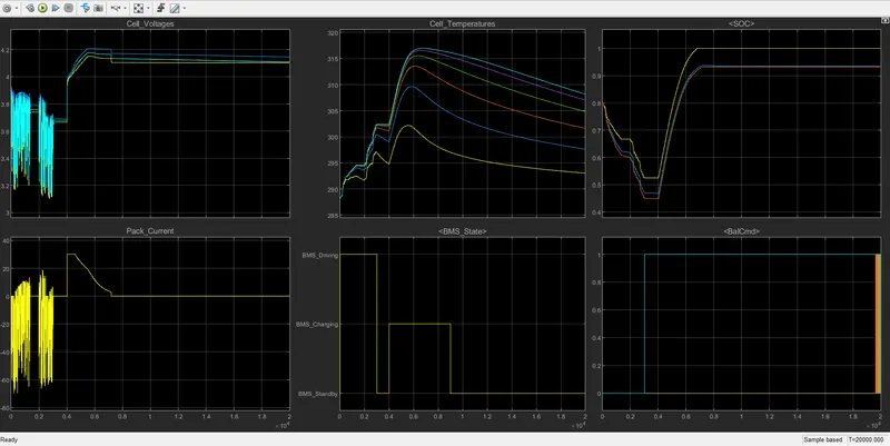
Cell voltage and peak current:-

As all the lamp indicators shows green, the system is free of faults. And let us understand the indiviual plots as follows:-

As we see, for the first 3000 seconds driving happens and hence the discharging is happpening for all the 6 cells. And the voltage is varied from 3.1 to 3.9V.

And from 3000 to 4000 seconds, the balancing occurs and hence the voltage is maintained as constant throughout this period.

After 4000 seconds, the charging happens and hence the voltage is again raised to around 4V and at constant current. And after when the maximum voltage is reached, we can see the downfall in the current and then the charging and balancing occurs for the next 9000 seconds.

Effect in cell temperatures:-

Initially for the first 3000 seconds the temperature is gradually rising from the 290K to 303 K approximately. Also as we noticed, the temperature of the cell 1 is lesser than the other 5 cells.

And from the 3000 to 4000 seconds, there no much changes in the current plots because of the balancing taking place.

After 4000 seconds, the temperature starts increasing exponentially till the constant current region and starts depleating in constant voltage and in cell balancing region.

At 9000 seconds, the temperatute further reduces and again attains the ambient tempperature range.

SOC:-

Here the SOC is determined with the help of the couloumb counting, UKF kalman filter and EKF kalman filter, which are referred as dofferent colour styles in the graph. As we can noticed clearly, By couloumb counting ie., from the results of yellow curve, the SOC is estimated as 100% and as per UKF & EKF kalman filters, the SOC is observed as 93% approximately . This is how the SOC is determined for the given discharging conditions.

Cell balancing:-

Initially upto 3000 seconds, the cell balancing is not activated, and after the 3000th second the balancing starts with cell number 6 and 2 as they attains a sudden creep in the graph, since its voltage is higher than the other.

Similarly in the cell number 1 which have the lesser voltage when compared with the other cell is maintained as same level throughout the stimulation. And hence at the end all the cells are in the balancing state.

TEST 2:-

For Test 2, the Test variant sequence is chosen as 2.

And for the 2nd test sequence, the following conditions are considered:-

Now when we run the stimulation, the following outputs will occur.

OUTPUT FOR TEST CASE 2:-

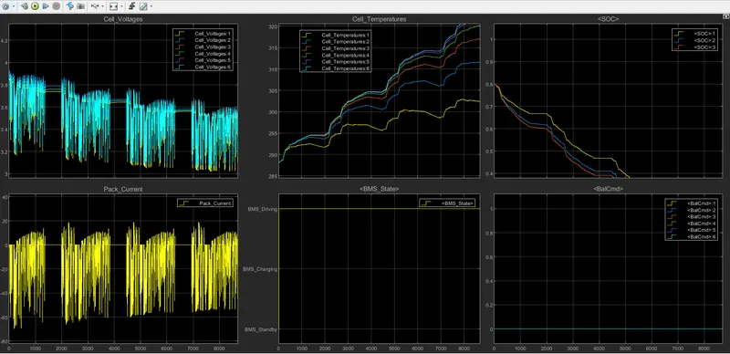
Here as we look into the test sequence, only driving ie., discharging takes place. And hence the cell temperatures are raising gradually from around 280K to 320k and since it is a continous discharging state, the SOC is reduced from 80% to 0%. As we also see that the cell voltage and the peak current is also reduced.

The cell balancing is not done here and hence we can experience a constant 0 vaalue in the cell balancing graph.

TEST 3:-

Here in the test sequence variant, number 3 is selected.

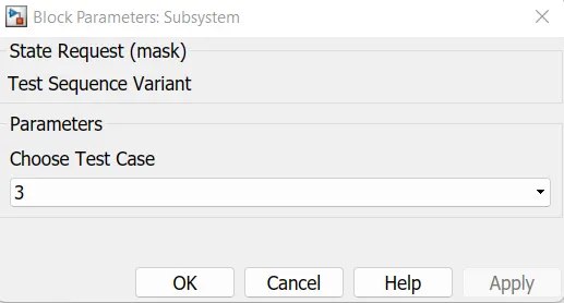
The following condition is used in this test 3 condition:-

OUTPUT FOR TEST CASE 3:-

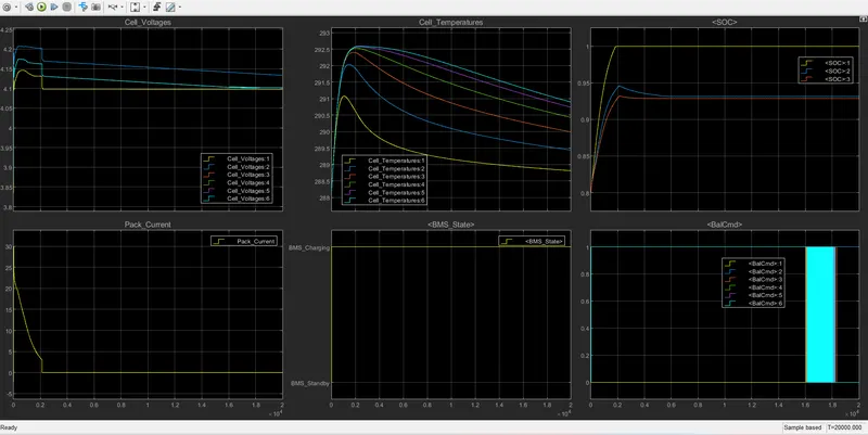
From the condition its clear that this is a Charging condition.

Cell voltage and peak current:-

When you look into the cell voltage and the peak current, we can find the constant current and constant voltage state of the battery. As we see, initially the cell voltage is raised to 4.2V and the current upto 30A and then the CC & CV modes starts. And hence we can see a straight constant line from the 0.2 seconds in the cell voltage and the ppeak current graph.

Effect in cell temperatures:-

The cell temperatures initially raised from 289K to 292.5K and from the 0.2 second the constant current and voltage flow takes place and hence the temperature of the cell drop again to the ambient temperature ie., around 288K.

SOC:-

The initial SOC is about 80% and after the 0.2seconds, the SOC is increased to about 100 % since constant charging takes place.

And hence from couloumb counting, the SOC is founf as 100% and from UKF , EKF kalman filter, the SOC is found to be 93% respectively.

-----------------------------------------------------------------------------------------------------------

Objective 2:-

Coulomb counting:-

SoC Estimation by Coulomb Counting is based on the measurement of the current and integration of that current over time.

The Coulomb counting method measures the discharging current of a battery and integrates the discharging current over time in order to estimate SOC.

Coulomb counting gives a relative change in SoC and not an absolute SoC. If you measure the current over a given time step you have a measure of the number of Ah that have left or been received by the battery.

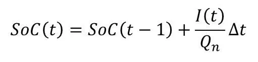
where:

• SoC(t) = estimated State of Charge at time, t
• SoC(t-1) = previous State of Charge at time t-1
• I(t) = charging or discharging current at time, t
• Q_n = battery cell capacity
• Δt = time step between t-1 and t

If you want to know the absolute SoC you need to know the starting SoC of the cell, SoC(t-1) as given in the equation. One option is to fully charge the cell to a known voltage. Charging to maximum cell voltage and SoC can be used as a reset and known point.

How BMS implements coulomb counting for SOC estimation in the avove model?

Double click the BMS ECU and open the SOC estimation block and then open the Coulomb counting block. The block willl appear as follows:-

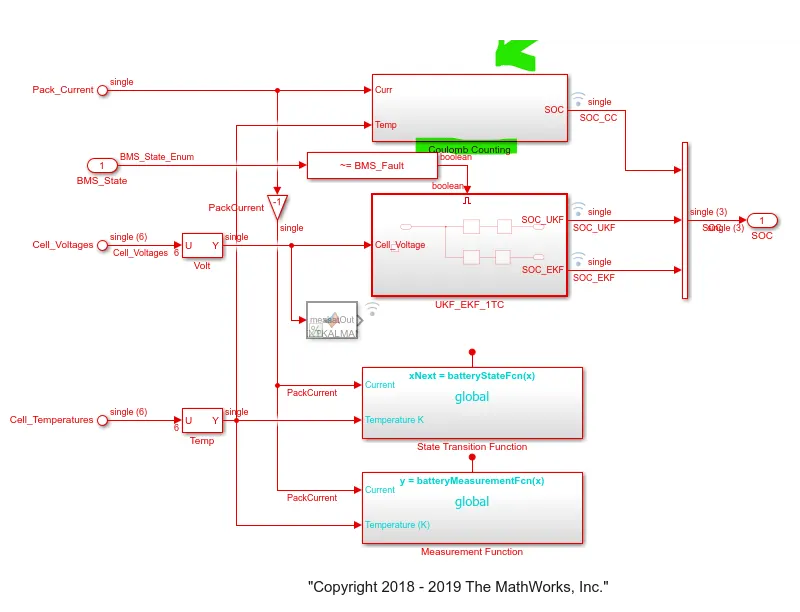
Now open the Coulomb counting block:-

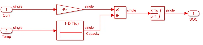
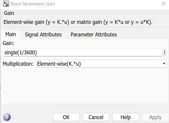
Here the discharge current from battery given to gain with value as 1/3600 to convert current to Amphere hour.

The value is divided by capacity due to temperature change. Then integrated with a gain value of 1 with sample time -1 as we are using discrete integrator.

The saturation limits are from 0 to 1.

We will get the SOC values from 0 to 1 multiplied with 100 to get in percentage of SOC.

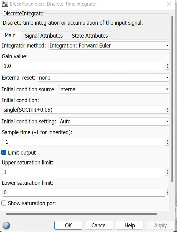
By this way the SOC is calculated for the above taken model.

Note:- The .slx files of R2019b is added in the answer box