Aim:
To solve the otto cycle using the matlab to get the PV diagram and to find out its thermal efficiency.
Software used:
Matlab R2022a
Description of the Project:
An Otto cycle is an idealized thermodynamic cycle that describes the functioning of a typical spark ignition piston engine. Now in this project we script the coding in matlab to find its PV-diagram for the given conditions and also to find its efficiency.
Before getting into our problem, we need to know how does an otto cycle works and also its quite important to know its 4 stages of working. This can be easily understoood by the drawing giveb below:
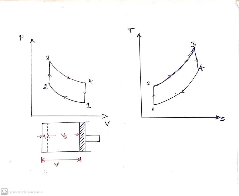
Process 1-2 => Isentropic compression
Process 2-3 => Constant volume heat addition
Process 3-4 => Isentropic expansion
Process 4-1 => Constant volume heat rejection
Compression ratio:
The compression ratio(r) is defined as the ratio of the volume at the bottom dead center and the volume at the top dead center. ie.,(v1/v2)
Now, From the Process 1-2,
T2/T1=(V1/V2)^γ-1
ie;
T2/T1=(r)^γ-1---------------------- (1)
similarly, From the process 3-4,
T3/T4=(V4/V3)^γ-1
ie.,
T3/T4=(r)^γ-1 [since, from the PV diagram, V1=V4 & V2=V3 ------------ (2)
Note:
We have to face two types of volumes inside the cylinder. one is swept volume( Vs) and the clearance volume (Vc). and hence the compression ratio can be defined as:
r=1+(Vs/Vc)
Vs= π/4*l*d^2---------------- (3)
here, l= stroke of the cylinder
d= Bore diameter
Also, from the derivation of compression ratio, we can obtain the clearance volume as,
Vc=Vs/(r-1)------------------ (4)
Also from the above diagram we know that,
V1=Vs+Vc --------------------- (5)
V2=Vc --------------------------(6)
Now let us see the matlab program and the different state variables will be explained in between the program codes:
EXPLAINATION OF CODES:
PROGRAM 1:
% state1 variables (given)
p1=101325
t1=500
t3=2300
These four lines determines the input for our air standard cycle
%engine parameters
bore=0.1
stroke=0.1
connecting_rod=0.15
r=12
After mentioning the inputs, the important engine parameters are defined inside the program. The bore,stroke and compression ratio are explained in the description.
% formula to find the sewpt volume and clearance volume
swept_vol=(pi/4)*bore^2*stroke
clear_vol=(swept_vol)/(r-1)
v1=swept_vol+clear_vol
v2=clear_vol
As discussed in equations (3) and (4), the equations of clearance volume,swept volume,v1& also v2 given in these above lines.
Now the next step is to attain all the process state points and when we plot it inside the graph, we will get our required output.
State points 1:- P1&T1 are given to us, and the value of V1 is taken from equation (5)
State points 2:-
To find P2: We know that, P1*V1^γ=P2*V2^γ
therefore, P2= P1*r^γ [ since, V1/V2=r ] ------------------------- (7)
To find T2: WKT, P1*V1/T1 = P2*V2/T2
therefore, T2= T1*(P2*V2/P1*V1) ------------------------------- (8)
For state points 3:
We know, V3=V2
Also, T3= 2300 ( given )
To calculate P3, we know that P2*V2/T2 = P3*V3/T3
therefore, P3= (P2*T3)/T2 --------------------------------- (9)
For state points 4:
We know, V4=V1 (from PV diagram)
also, T4=T3 (from TS diagram)
To find P4, WKT P3*V3^γ=P4*V4^γ
therefore, P4= P3*(V3/V4)^γ ------------------------------ (10)
Now from the above explained steps,
% TO FIND THE VARIABLES @ state 2 (ie., p2,v2,t2)
% (i) To find p2&t2
% we knw that, p1v1^gamma=p2v2^gamma
%input
gamma=1.4
p2=p1*r^gamma;
t2=t1*p2*v2/(p1*v1)
% TO FIND THE VARIABLES @ state 3 (ie., p3,v3,t3)
v3=v2
p3=p2*t3/t2
% TO FIND THE VARIABLES @ state 4 (ie., p4,v4,t4)
v4=v1
%also wkt, p3v3^gamma=p4v4^gamma( therefore,)
p4=p3*(v3/v4)^gamma
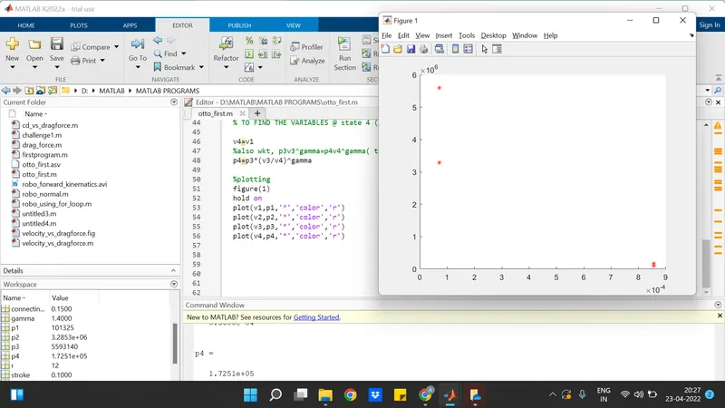
And then the values of v1,p1, v2,p2, v3,p3, v4,p4 are plotted in the grapg using the 'plot' code as follows:
figure(1)
hold on
plot(v1,p1,'*','color','r')
plot(v2,p2,'*','color','r')
plot(v3,p3,'*','color','r')
plot(v4,p4,'*','color','r')
Now the output for the plots will come as follows:
EXPLAINATION OF CODES:
PROGRAM 2: Engine Kinematics
This program is assigned as a template for our initial program and hence we are going to define our function statement here and it comes as follows:
function[V]=engine_kinematics(bore,stroke,connecting_rod,r,start_crank,end_crank)
This is our function statement, Which consists of all our engine specifications, such as bore,stroke etc.,
Now the following formula is used to determine, how thw volume inside the combustion engine is going to change for the respective crank angles:
V/Vc= 1+ 0.5(r-1)[R+1-cosθ-(R^2-sin^2θ)^0.5
This formula is seperated as terms1,2&3 for easu calculation purpose and the 'linspace' code is used to provide different θ values and defined in matlab as follows:
theta=linspace(start_crank,end_crank,100);
term1=0.5*(r-1);
term2=R+1-cosd(theta);
term3=(R^2-sind(theta).^2).^0.5;
And the following lines represent the inputs for R & a
a=stroke/2;
R=connecting_rod/a;
And the three terms are merged and our final formula for V will look like as follows :
V=(1+term1*(term2-term3)).*clear_vol;
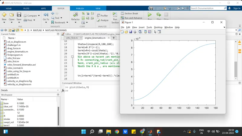
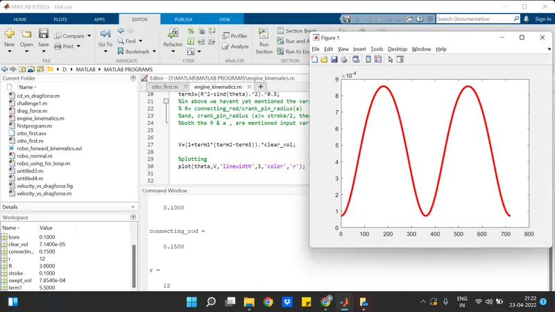
using the 'end' code, end the function. Now when you plot the graph for the different theta values against V, you will get the following outputs:
These are the two outputs for the volume traces.
EXPLAINATION OF CODES:
CALLING THE FUNCTION:-
constant_c=p1*v1^gamma
V_compression=engine_kinematics(bore,stroke,connecting_rod,r,180,0);
constant_c=p3*v3^gamma
V_expansion=engine_kinematics(bore,stroke,connecting_rod,r,0,180);
P_expansion=constant_c./V_expansion.^gamma;
P_compression=constant_c./V_compression.^gamma;
By using the above codes, the constant is defined, and also the function is called from the engine_kinematics program and the different values for P&V, compression and expansions are found out and then they are plotted.
%plotting
figure(1)
hold on
plot(v1,p1,'*','color','r')
plot(V_compression,P_compression)
plot(v2,p2,'*','color','r')
plot([v2,v3],[p2,p3])
plot(v3,p3,'*','color','r')
plot(V_expansion,P_expansion)
plot(v4,p4,'*','color','r')
plot([v4,v1],[p4,p1])
xlabel('Volume')
ylabel('Pressure')
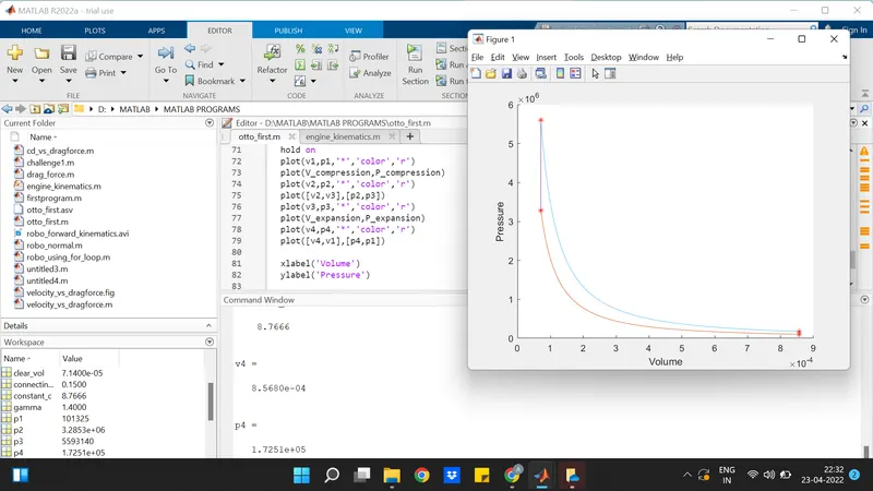
Finally the plotting for all the expansion and compression points are done with the help of the above syntax codes. And the final output will look as follows:-
TO FIND THE EFFICIENCY:
% To calculate thermal efficiency
efficiency=(1-(1/r^(gamma-1)))*100
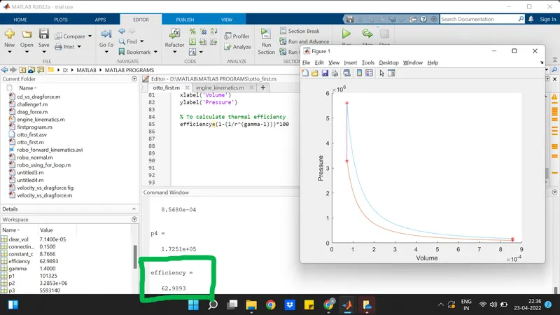
The above formula is used to calculate the termal efficiency of the otto cycle and is calculated as follows:
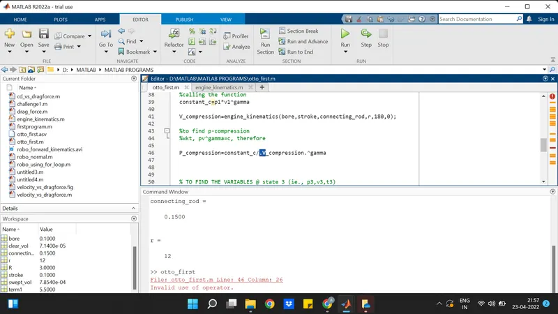
ERRORS MADE WHILE PROGRAMMING:-
- Missing the comma, for the asterisk symbol plot
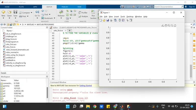
ii. Done a mistake while typing the element wise operator
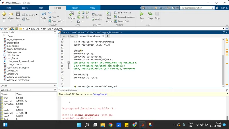
iii. Unrecognizing the variable by defining it after the formula
iv. Unknowingly giving brackets to the line width value
Things done to overcome errors:
Refered the videos onceagain and also corrected with thw help of the practice and E-book.
OUTPUTS:
EFFICIENCY OUTPUT WITH THE PV- DIAGRAM:
PV- DIAGRAM OUTPUT:
PROGRAM TO FIND OUT THE PV DIAGRAM FOR THE OTTO CYCLE AND ALSO TO FIND ITS EFFICIENCY:
%PROGRAM TO FINDOUT THE PV DIAGRAM & THERMAL EFFICIENCY FOR AN AIR STANDARD CYCLE

clear all
close all
clc

% state1 variables (given)

p1=101325
t1=500
t3=2300

%engine parameters

bore=0.1
stroke=0.1
connecting_rod=0.15
r=12

% formula to find the sewpt volume and clearance volume

swept_vol=(pi/4)*bore^2*stroke
clear_vol=(swept_vol)/(r-1)
v1=swept_vol+clear_vol
v2=clear_vol

% TO FIND THE VARIABLES @ state 2 (ie., p2,v2,t2)

% (i) To find p2&t2
% we knw that, p1v1^gamma=p2v2^gamma

%input
gamma=1.4

p2=p1*r^gamma;

% Also wkt, p1v1/t1 = p1v1/t2
t2=t1*p2*v2/(p1*v1)

%calling the function
constant_c=p1*v1^gamma

V_compression=engine_kinematics(bore,stroke,connecting_rod,r,180,0);

%to find p-compression
%wkt, pv^gamma=c, therefore

P_compression=constant_c./V_compression.^gamma;


% TO FIND THE VARIABLES @ state 3 (ie., p3,v3,t3)

v3=v2
% Also wkt, p2v2/t2= p3v3/t3 {since, v3=v3, they cancel each other}
p3=p2*t3/t2

constant_c=p3*v3^gamma

V_expansion=engine_kinematics(bore,stroke,connecting_rod,r,0,180);

P_expansion=constant_c./V_expansion.^gamma;


% TO FIND THE VARIABLES @ state 4 (ie., p4,v4,t4)

v4=v1
%also wkt, p3v3^gamma=p4v4^gamma( therefore,)
p4=p3*(v3/v4)^gamma

%plotting
figure(1)
hold on
plot(v1,p1,'*','color','r')
plot(V_compression,P_compression)
plot(v2,p2,'*','color','r')
plot([v2,v3],[p2,p3])
plot(v3,p3,'*','color','r')
plot(V_expansion,P_expansion)
plot(v4,p4,'*','color','r')
plot([v4,v1],[p4,p1])

xlabel('Volume')
ylabel('Pressure')

% To calculate thermal efficiency
efficiency=(1-(1/r^(gamma-1)))*100
PROGRAM TO FIND OUT THE ENGINE KINEMATICS ( FUNCTION PROGRAM):
%PROGRAM TO FIND OUT THE ENGINE KINEMATICS


function[V]=engine_kinematics(bore,stroke,connecting_rod,r,start_crank,end_crank)


a=stroke/2;
R=connecting_rod/a;

swept_vol=(pi/4)*bore^2*stroke;
clear_vol=(swept_vol)/(r-1);

theta=linspace(start_crank,end_crank,100);

term1=0.5*(r-1);
term2=R+1-cosd(theta);
term3=(R^2-sind(theta).^2).^0.5;
%in above we havent yet mentioned the variable R
% R= connecting_rod/crank_pin_radius(a)
%and, crank_pin_radius (a)= stroke/2, therefore
%both the R & a , are mentioned input variables above


V=(1+term1*(term2-term3)).*clear_vol;

end