Week 3 - Solving second order ODEs

Solving the ODE for the simple pendulum and to create the animation of the pendulum

Aim:

To solve a second order ODE of a simple pendulum and also to create its animation using Matlab

Software used:

MATLAB R2022a

Project Description:

Order of an ODE:

The order of a differential equation is defined to be that of the highest order derivative it contains. The degree of a differential equation is defined as the power to which the highest order derivative is raised.

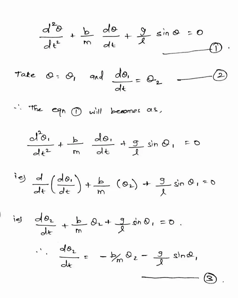
Here in our project, we will solve an differential equation of an simple pendulum which have some displacement and velocity, which varies with time. The differential equation of the simple pendulum is given as:

Here the highest power in the above equation is two and hence it will be termed as second order differential equation. Also in the above euation,

g = gravity in m/s2,

L = length of the pendulum in m,

m = mass of the ball in kg,

b=damping coefficient.

Solving the ODE:

Program and its Explainations:

To solve the differential equation of a pendulum, initially a function program has been written and the function calling had been done in the main program for the respective angular displacement (θ) values. The function program will be coded as follows:-

• Function Program explaination:

• Main Program explaination:

The first few coding lines are used to introduce our variables, which are our inputs for our pendulum

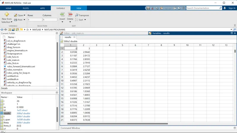
Now in our results segment , we will get two coloumn matrix, in which the first coloumn represents the Displacements and the second coloumn represent the velocity values as follows:-

%plotting

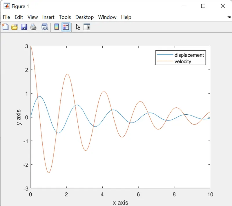
Now the plotting for the obtained displacment and velocity values are plotted against the time.

figure(1)

plot(t,results(:,1)) -----> This code is used to plot the 't' value & the first coloumn(ie.,displacement) of the results sheet.

hold on ----->'hold on' code is used to hold the plot since we are using more than one 'plot' commands

plot(t,results(:,2)) ------> The next 'plot' code is used to plot the 't' values and the second coloumn(ie.,velocity) of the results sheet

xlabel('x axis')

ylabel('y axis')

legend({'displacement','velocity'}) -----> 'legend' code is used to give the explainantion for colours and which the curve belongs to.

Now when we run the progran, we will get the output for the given inputs, and the graph is plotted for the displacement and velocity curves which changes with respect to the time.

OUTPUT 1:

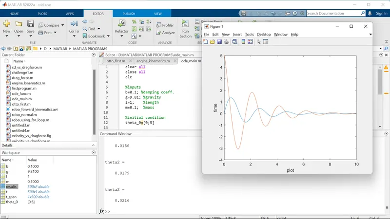
Now when you reduce your damping value, ie .,b value you will get the output accordingly

Creating a for loop to ontain the animation of the simple pendulum:

Now before creating the 'for' loop, we have to give its input to the for and hence the above coding line, the first coloumn of results sheet, is getting stored in a variable called theta. That is what represented as results(:,1)

Then the following lines are used to create the animation. The videofile is created and it is saven in the format of uncompressed avi. Then the video is getting write and then we can close the video file.

Now when you run the program, we will get the output as the animated pendulum & it looks as follows:

OUTPUT:

YOUTUBE LINK : https://youtu.be/VoslAvoWXUM

FUNCTION PROGRAM:-

%FUNCTION PROGRAM


function[dtheta_dt]=ode_func(t,theta,b,g,l,m)
theta1=theta(1);
theta2=theta(2)
dtheta1_dt=theta2;
dtheta2_dt=-(b/m)*theta2-(g/l)*sin(theta1);
dtheta_dt=[dtheta1_dt;dtheta2_dt];
end

MAIN PROGRAM:-

clear all
close all
clc

%inputs
b=0.05; %damping coeff.
g=9.81; %gravity
l=1;    %length
m=0.1;  %mass

%initial condition of Displacement & velocity
theta_0=[0;3]

%timespan
t_span=linspace(0,10,500);

%solving ode & calling the function
[t,results]= ode45(@(t,theta) ode_func(t,theta,b,g,l,m),t_span,theta_0);

%plotting 
figure(1)
plot(t,results(:,1)) %plotting the 1st coloumn of results sheet with time
hold on
plot(t,results(:,2)) %plotting the 2nd coloumn of results sheet with time
xlabel('x axis')
ylabel('y axis')
legend({'displacement','velocity'})

%To create the for loop Pendulum Animation

theta=results(:,1) % first coloumn of results ie.,angular displacement
ct=1;              %counter variable


for i=1:length(theta)

%starting position of the string

    x1=0
    y1=2
    
%position of the bob

  x2=-l*sin(theta(i));
  y2=-l*cos(theta(i));

  figure(2)
  plot([-1.5,1.5],[2,2],'color','r',LineWidth=3)
  hold on
  plot([x1,x2],[y1,y2],LineWidth=3)
  plot(x2,y2,'o',MarkerSize=30,MarkerFaceColor='black',MarkerEdgeColor='green')
  hold off
  xlim([-2.5,2.5])
  ylim([-2.5,2.5])
  title('Animation of a Simple Pendulum')
  pause(0.1)
  M(ct)=getframe(gcf);
  ct=ct+1
end

%To create the Animation

videofile=VideoWriter('pendulum animation.avi','Uncompressed AVI');
open(videofile);
writeVideo(videofile,M)
close(videofile)

ERRORS FACED :-

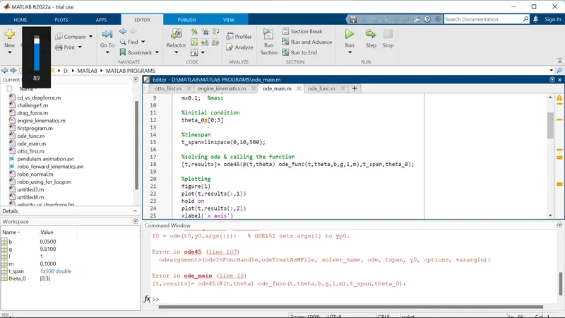
1) Unknowingly made a comma in the function statement in the function program, so that my main program got stucked with throwing error.

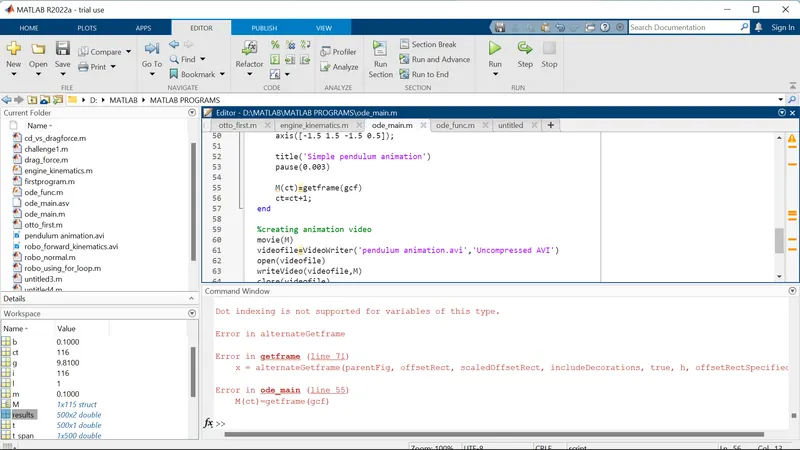
2) Closing the animation before it got ended will get you an error in 'getframe' code and your video will not get saved in your folder.

Steps to overcome the errors:-

I found a little difficult to find out the 2nd error ie.,in the 'getframe' code. so i sheduled a one on one session and got all my doubts cleared.

OUTPUT OF PENDULUM ANIMATION:

YOUTUBE LINK: https://youtu.be/VoslAvoWXUM