Week 4.1 - Genetic Algorithm

Optimization of Mathematical Stalagmite function using Genetic Algorithm

Aim:

To write a code to optimize the stalagmite function and to find out the local maxima with the help of genetic algorithm

Software used:

MATLAB R2022a

Project Description:

Stalagmite:-

A stalagmite is an upward-growing mound of mineral deposits that have precipitated from water dripping onto the floor of a cave. Most stalagmites have rounded or flattened tips.

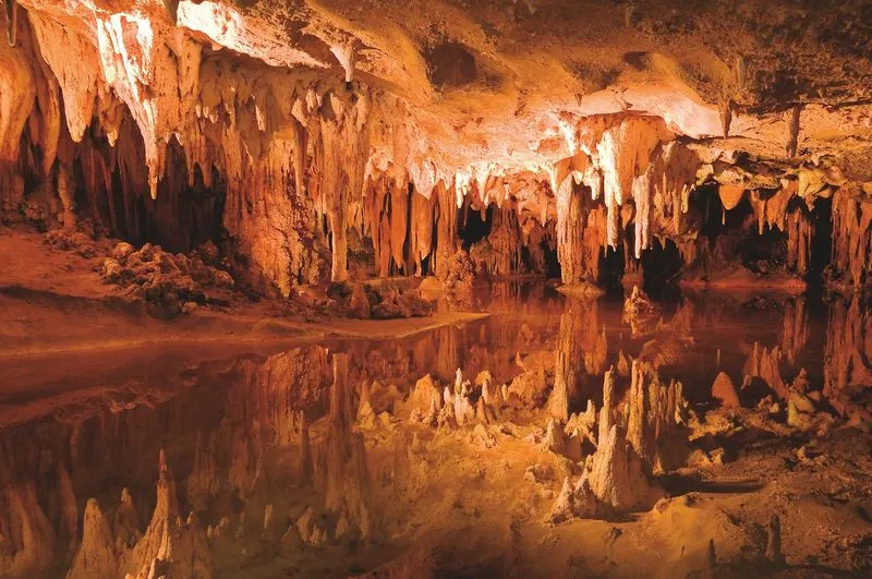
Now here in our project, we are going to find a mathematical model for this stalagmite function with the help of the genetic algorithm using matlab and also we are going to find out the global maxima or minima. And for that we need to know about the concept of genetic algorithm and that can be explained as follows:-

Genetic Algorithm:-

The genetic algorithm is a method for solving both constrained and unconstrained optimization problems that is based on natural selection, the process that drives biological evolution. The genetic algorithm repeatedly modifies a population of individual solutions.A genetic algorithm is a search heuristic that is inspired by Charles Darwin’s theory of natural evolution. This algorithm reflects the process of natural selection where the fittest individuals are selected for reproduction in order to produce offspring of the next generation.

Optimization techniques are the techniques used to discover the best solution out of all the possible solutions available under the constraints present. The genetic algorithm is one such optimization algorithm built based on the natural evolutionary process of our nature. The idea of Natural Selection and Genetic Inheritance is used here. Unlike other algorithms, it uses guided random search, i.e., finding the optimal solution by starting with a random initial cost function and then searching only in the space with the least cost (in the guided direction). Suitable when you are working with huge and complex datasets.

Five phases are considered in a genetic algorithm.

1. Initial population
2. Fitness function
3. Selection
4. Crossover
5. Mutation

1)Initial polulation:-

The process begins with a set of individuals which is called a Population. Each individual is a solution to the problem you want to solve.

2)Fitness Function:-

The fitness function determines how fit an individual is (the ability of an individual to compete with other individuals). It gives a fitness score to each individual. The probability that an individual will be selected for reproduction is based on its fitness score.

3)Selection:-

The idea of selection phase is to select the fittest individuals and let them pass their genes to the next generation.Two pairs of individuals (parents) are selected based on their fitness scores. Individuals with high fitness have more chance to be selected for reproduction.

4)Crossover:-

Crossover is the most significant phase in a genetic algorithm. For each pair of parents to be mated, a crossover point is chosen at random from within the genes.

5)Mutation:-

In certain new offspring formed, some of their genes can be subjected to a mutation with a low random probability. This implies that some of the bits in the bit string can be flipped.Mutation occurs to maintain diversity within the population and prevent premature convergence.

The following image will helps us to understand the concept of genetic algorithm in a better manner:-

Our given stalagmite function:-

Now with the enough knowledge of stalagmite and the genetic algorithm, we will get inside our program proceedings:-

In this project we are provided with a stalagmite function represented as follows:

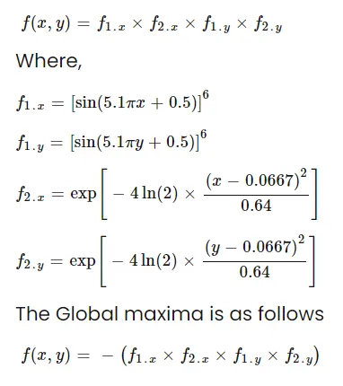
Here the usage of ga is to find out the local minima. But in our case, we need to find out the local maxima. And hence what we do is, we just invert the function formula with a negative sign.

And hence for this function of f(x,y), we are going to derive the mathematical stalagmite model as follows:-

Function program and its Explainations:-

Here in the function program named 'stalagmite', contains the function f with 'input_vector' as the function definition and that is stored in two variables x and y.

Then the total function is divided into four terms as f1x, f1y, f2x, f2y and the final function have been arrived by the product of these four terms and is given in the last line of the program.

The negative sign in the function indicates that the function is inverted to find out the local maxima value.

FUNCTION PROGRAM:-

%Function program for stalagmite

function [f]=stalagmite(input_vector)

x=input_vector(1);
y=input_vector(2);

f_1x=((sin(5.1*pi*x+0.5))^6);
f_1y=((sin(5.1*pi*y+0.5))^6);
f_2x=exp(-4*log(2)*((x-0.0667).^2)./0.64);
f_2y=exp(-4*log(2)*((y-0.0667).^2)./0.64);
[f]=-(f_1x*f_1y*f_2x*f_2y);

end

MAIN PROGRAM TO DEFINE THE STALAGMITE FUNCTION WITH THE HELP OF GA & ITS STEP BY STEP EXPLAINATIONS:-

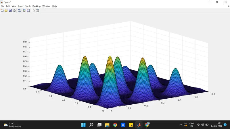
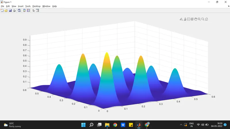
In the above codes, we are defining the values of x and y with the help oh 'linspace' code which creates 150 values between 0 & 0.6.

And the 'meshgrid' code is used to obtain the surface plots as grid for the obtained x and y values.

for i=1:length(xx)

for j=1:length(yy);

input_vector(1)=xx(i,j);

input_vector(2)=yy(i,j);

f(i,j)=stalagmite(input_vector);

end

end

surfc(xx,yy,-f)

The negative sign is used for inverting the surface

Then, we are going to generate a loop for the obtaied grid values of xx and yy, and are get stored in the varoalbles called input_vector(1) & input_vector(2) and then the function value is called in the statement f(i,j)=stalagmite(input_vector)----> where 'stalagmite' is my function program, which we have discussed initially.

And when I try to plot the xx,yy&f values using the 'surfc' code, I will get a an output as follows:-

To get a smooth surface, 'shading interp' code is used, and we get the results as:

And then we are going to witness the statistical behaviour of the genetic algorithm using the 'ga' code. And for that wee need to know about the syntax of ga. That can be explained as follows:

----------------------------------------------------------------------------------------------------------------------------------------------------------------------------------------------------

********************************************************************************************************************************************

Syntax for 'ga':-

1. x = ga(fun,nvars)
2. x = ga(fun,nvars,A,b)
3. x = ga(fun,nvars,A,b,Aeq,beq)
4. x = ga(fun,nvars,A,b,Aeq,beq,lb,ub)
5. x = ga(fun,nvars,A,b,Aeq,beq,lb,ub,nonlcon)
6. x = ga(fun,nvars,A,b,Aeq,beq,lb,ub,nonlcon,options)
7. x = ga(fun,nvars,A,b,Aeq,beq,lb,ub,nonlcon,intcon)
8. x = ga(fun,nvars,A,b,Aeq,beq,lb,ub,nonlcon,intcon,options)
9. x = ga(problem)

Description for the above syntax:

1. x = ga(fun,nvars) finds a local unconstrained minimum, x, to the objective function, fun. nvars is the dimension (number of design variables) of fun.
2. x = ga(fun,nvars,A,b) finds a local minimum x to fun, subject to the linear inequalities A*x ≤ b. ga evaluates the matrix product A*x as if x is transposed (A*x').
3. x = ga(fun,nvars,A,b,Aeq,beq,lb,ub) defines a set of lower and upper bounds on the design variables, x, so that a solution is found in the range lb ≤ x ≤ ub. (Set Aeq=[] and beq=[] if no linear equalities exist.)
4. x = ga(fun,nvars,A,b,Aeq,beq,lb,ub,nonlcon) subjects the minimization to the constraints defined in nonlcon. The function nonlcon accepts x and returns vectors C and Ceq, representing the nonlinear inequalities and equalities respectively. ga minimizes the fun such that C(x) ≤ 0 and Ceq(x) = 0. (Set lb=[] and ub=[] if no bounds exist.)
5. x = ga(fun,nvars,A,b,Aeq,beq,lb,ub,nonlcon,options) minimizes with the default optimization parameters replaced by values in options. (Set nonlcon=[] if no nonlinear constraints exist.) Create options using optimoptions.
6. x = ga(fun,nvars,A,b,Aeq,beq,lb,ub,nonlcon,intcon) or x = ga(fun,nvars,A,b,Aeq,beq,lb,ub,nonlcon,intcon,options) requires that the variables listed in intcon take integer values.
7. x = ga(problem) finds the minimum for problem, a structure described in problem.

*******************************************************************************************************************************************

num_cases=50;

%study 1- STUDY OF STATISTICAL BEHAVIOUR OF GA

for i=1:num_cases

[inputs,fopt(i)]=ga(@stalagmite,2);

xopt(i)=inputs(1);

yopt(i)=inputs(2);

end

Here in the above codes, the number of itreations has been set as 50 and the loop os activated for the set of itreations and by using the code 'ga' the function and the number of variabled are mentioned and the inputs(1) & inputs(2) are saved in the xopt and yopt (optimum) values.

figure(1)

subplot(2,1,1);

surf(x,y,-f);

shading interp

hold on

plot3(xopt,yopt,-fopt,'marker','o','MarkerSize',5,'MarkerFaceColor','r');

title('Unbounded Inputs');

subplot(2,1,2);

plot(fopt);

xlabel('Iterations');

ylabel('Function Minimum');

Then the plotting is done for the generated ga for the given number of itreations with the subplots and we will get the output as follows:-

And here we can see that the intreation values are unbounded and we are not getting an optimum value. So now we will try to bound the function within some limits and then use the 'ga' code to run the program and the script will fall as follows:-

%study 2- Stastical behaviour of ga with upper and lower bounds

tic

for i=1:num_cases;

[inputs,fopt(i)]=ga(@stalagmite,2,[],[],[],[],[0;0],[0.4;0.4]); -------> The syntax (iv) is used to define the 'ga' (Refer the syntax- iv mentioned above)

xopt(i)=inputs(1);

yopt(i)=inputs(2);

end

study_time2=toc ----------> The 'tic & toc' code is used to find out the time taken for processing the itreation values.

And here the 'ga' is defined with the help of some lower and upper bounds and hence out values will get optimized further and we will get a little more optimized results for the given number of itreations. And when we run the code, we will get the output as follows:-

%plotting the study 2

figure(2)

subplot(2,1,1);

surf(x,y,-f);

shading interp

hold on

plot3(xopt,yopt,-fopt,'marker','o','MarkerSize',5,'MarkerFaceColor','r');

title('Unbounded Inputs');

subplot(2,1,2);

plot(-fopt);

xlabel('Iterations');

ylabel('Function Minimum');

OUTPUT:-

As you can see, the in the above image, the values are further more optimized and they fall inbetween the defined upper and lower bounds.

Now to optimize more, the next step we are going to do is by increasing the population size. And we can witness a further more optimized model when we increase the population cound and the script will comes as follows:-

%study-3 Increasing the polpulation size

options=optimumoptions('ga');

options=optimumoptions(options,'populationsize',400); ----------> Mentioning the size of the population by using the syntax (v) mentioned above

tic

for i=1:num_cases;

[inputs,fopt(i)]=ga(@stalagmite,2,[],[],[],[],[0;0],[0.4;0.4],[],[],options); ------> Syntax (v) is used

xopt(i)=inputs(1);

yopt(i)=inputs(2)

end

study_time3=toc

And here in the above lines of codes, we are increasing the population size in the ga by using the syntax (v) mentioned above. Now when we increace the population count by 400, the ga will get optimized even further and most probably our local maxima and minima values can be foud out. Now plotting can be done by the help of the following codes:

figure(3)

subplot(2,1,1);

surf(x,y,-f);

shading interp

hold on

plot3(xopt,yopt,-fopt,'marker','o','MarkerSize',5,'MarkerFaceColor','r');

title('Unbounded Inputs');

subplot(2,1,2);

plot(-fopt);

xlabel('Iterations');

ylabel('Function Minimum');

OUTPUT:-

And as we can see, the values are further optimized and we can get a global maxima value perfectly by increasing the population size.

MAIN PROGRAM WITH 3 STUDIES COMBINED:-

clear all
close all
clc

x=linspace(0,0.6,150);
y=linspace(0,0.6,150);

[xx yy]=meshgrid(x,y);


for i=1:length(xx)
    for j=1:length(yy);
    input_vector(1)=xx(i,j);
    input_vector(2)=yy(i,j);
    f(i,j)=stalagmite(input_vector);
    end
end
num_cases=50;

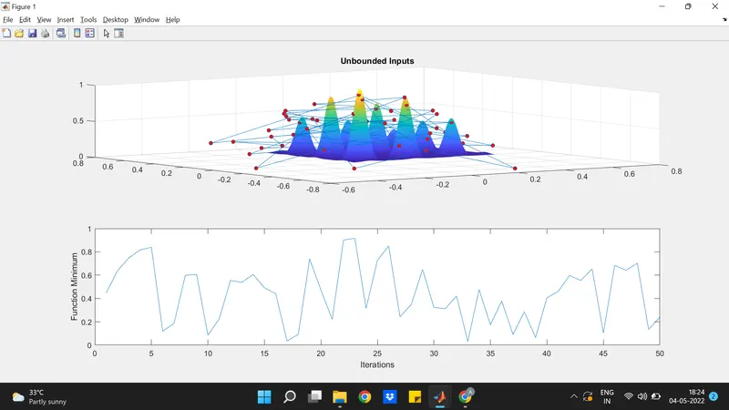
%study 1- STUDY OF STATISTICAL BEHAVIOUR OF GA
for i=1:num_cases
    [inputs,fopt(i)]=ga(@stalagmite,2);
    xopt(i)=inputs(1);
    yopt(i)=inputs(2);
end
figure(1)
subplot(2,1,1);
surf(x,y,-f);
shading interp
hold on
plot3(xopt,yopt,-fopt,'marker','o','MarkerSize',5,'MarkerFaceColor','r');
title('Unbounded Inputs');
subplot(2,1,2);
plot(-fopt);
xlabel('Iterations');
ylabel('Function Minimum');

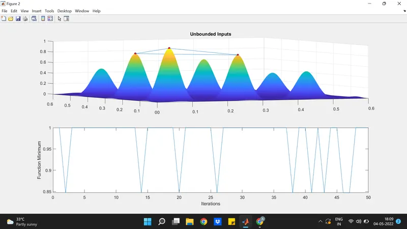
%study 2- Stastical behaviour of ga with upper and lower bounds

tic
for i=1:num_cases;
    [inputs,fopt(i)]=ga(@stalagmite,2,[],[],[],[],[0;0],[0.4;0.4]);
    xopt(i)=inputs(1);
    yopt(i)=inputs(2);
end
study_time2=toc

figure(2)
subplot(2,1,1);
surf(x,y,-f);
shading interp
hold on
plot3(xopt,yopt,-fopt,'marker','o','MarkerSize',5,'MarkerFaceColor','r');
title('Unbounded Inputs');
subplot(2,1,2);
plot(-fopt);
xlabel('Iterations');
ylabel('Function Minimum');

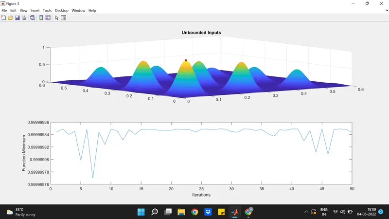
%study-3 Increasing the polpulation size

options=optimoptions('ga');
options=optimoptions(options,'populationsize',400);

tic
for i=1:num_cases;
    [inputs,fopt(i)]=ga(@stalagmite,2,[],[],[],[],[0;0],[0.4;0.4],[],[],options);
    xopt(i)=inputs(1);
    yopt(i)=inputs(2)
end
study_time3=toc

figure(3)
subplot(2,1,1);
surf(x,y,-f);
shading interp
hold on
plot3(xopt,yopt,-fopt,'marker','o','MarkerSize',5,'MarkerFaceColor','r');
title('Unbounded Inputs');
subplot(2,1,2);
plot(-fopt);
xlabel('Iterations');
ylabel('Function Minimum');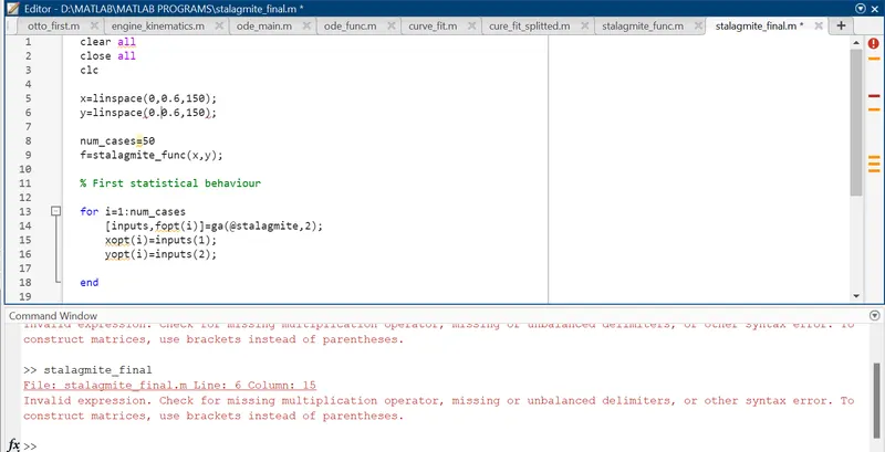

Errors Spotted:-

1) Unknowingly putting dot instead of comma in linspace code

References:-

1) https://in.mathworks.com/discovery/genetic-algorithm.html

2)https://towardsdatascience.com/introduction-to-genetic-algorithms-including-example-code-e396e98d8bf3

3)https://www.sciencedirect.com/topics/engineering/genetic-algorithm

4)https://skill-lync.com/student-projects/Genetic-algorithm-26340

5)https://skill-lync.com/student-projects/Stalagmite-function-67841

Function Program:-

%Function program for stalagmite

function [f]=stalagmite(input_vector)

x=input_vector(1);
y=input_vector(2);

f_1x=((sin(5.1*pi*x+0.5))^6);
f_1y=((sin(5.1*pi*y+0.5))^6);
f_2x=exp(-4*log(2)*((x-0.0667).^2)./0.64);
f_2y=exp(-4*log(2)*((y-0.0667).^2)./0.64);
[f]=-(f_1x*f_1y*f_2x*f_2y);

end

MAIN PROGRAM:-

clear all
close all
clc

x=linspace(0,0.6,150);
y=linspace(0,0.6,150);

[xx yy]=meshgrid(x,y);


for i=1:length(xx)
    for j=1:length(yy);
    input_vector(1)=xx(i,j);
    input_vector(2)=yy(i,j);
    f(i,j)=stalagmite(input_vector);
    end
end
num_cases=50;

%study 1- STUDY OF STATISTICAL BEHAVIOUR OF GA
for i=1:num_cases
    [inputs,fopt(i)]=ga(@stalagmite,2);
    xopt(i)=inputs(1);
    yopt(i)=inputs(2);
end
figure(1)
subplot(2,1,1);
surf(x,y,-f);
shading interp
hold on
plot3(xopt,yopt,-fopt,'marker','o','MarkerSize',5,'MarkerFaceColor','r');
title('Unbounded Inputs');
subplot(2,1,2);
plot(-fopt);
xlabel('Iterations');
ylabel('Function Minimum');

%study 2- Stastical behaviour of ga with upper and lower bounds

tic
for i=1:num_cases;
    [inputs,fopt(i)]=ga(@stalagmite,2,[],[],[],[],[0;0],[0.4;0.4]);
    xopt(i)=inputs(1);
    yopt(i)=inputs(2);
end
study_time2=toc

figure(2)
subplot(2,1,1);
surf(x,y,-f);
shading interp
hold on
plot3(xopt,yopt,-fopt,'marker','o','MarkerSize',5,'MarkerFaceColor','r');
title('Unbounded Inputs');
subplot(2,1,2);
plot(-fopt);
xlabel('Iterations');
ylabel('Function Minimum');

%study-3 Increasing the polpulation size

options=optimoptions('ga');
options=optimoptions(options,'populationsize',400);

tic
for i=1:num_cases;
    [inputs,fopt(i)]=ga(@stalagmite,2,[],[],[],[],[0;0],[0.4;0.4],[],[],options);
    xopt(i)=inputs(1);
    yopt(i)=inputs(2)
end
study_time3=toc

figure(3)
subplot(2,1,1);
surf(x,y,-f);
shading interp
hold on
plot3(xopt,yopt,-fopt,'marker','o','MarkerSize',5,'MarkerFaceColor','r');
title('Unbounded Inputs');
subplot(2,1,2);
plot(-fopt);
xlabel('Iterations');
ylabel('Function Minimum');