Week 7 State of charge estimation

Q1.Simulate the 3 test cases from harness dashboard and write a detailed report on the results

Ans1. We are provided with the BMS project model, which have 3 modes

1. Balancing

2. Charging

3. Drive

The whihc is used is given bellow:-

MODEL

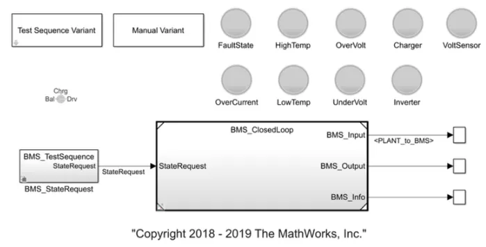
CASE 01

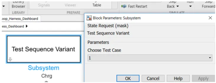
1)Click on the Test Sequence Varient Block and select test case as 1

TEST CASE

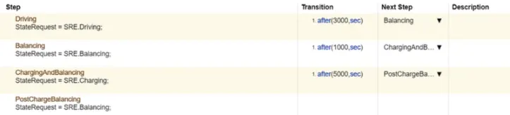
Now by clicking on the BMS Sequence block we get the chart

Sequence 1

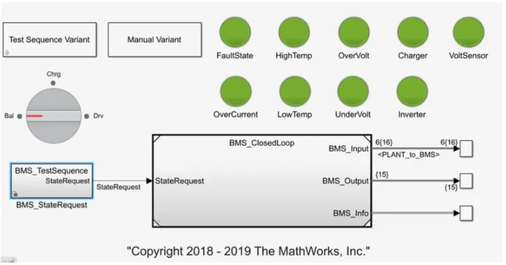
MODEL:-

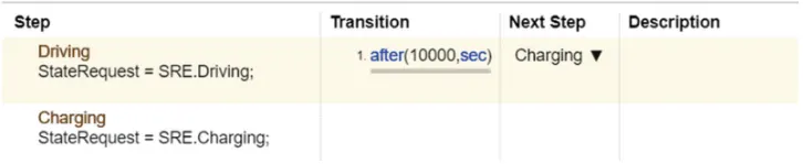
When simulation will start, the model will be in driving condition. After 3000 seconds it will be in standby mode and after 1000 seconds it will be in charging mode. Now by Running the simulation.

Result 1 :- Here all the indicators are green. So we can see no errors and we check the plot for this model and is shown below.

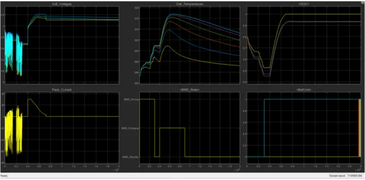
i) Driving (Discharging) mode (0-3000 sec):- All the cells for the first 3000 sec are in driving mode so the dicharge of all the cell occurs and its varies in the range of 3.1 to 3.9 V (min and max.).

Cell temprature increases from 288K to 302 K.

SOC also reduces from 80 % to 45% for EKF technique.

ii) Balancing mode (3000-4000 sec) :- After 3000sec for 1000 sec, cell balancing occur and the Modules are in standby mode and they are having constant voltage near about 3.7V.

Cell temperature reduces slowly as no current flow through the cells during balancing.

SOC is also constant during this period i.e. 45% for EKF technique.

iii) Charging and Balancing (4000- 9000 sec):- After 4000 sec the charging occurs and the cell voltages increased from 3.7 to nearly about 4.2 V in Constant current mode with current of nearly 30A and then the constant voltage charging starts and current reduces from 30A to 2.6 A Charging and balancing of cells occur till 9000 sec.

Cell temperature also start to increase exponentially upto constant current region and reduces as current flow reduces in constant voltage mode.

SOC also increases from 45% to 94% in this mode for EKF technique.

iv) Post charge Balancing (9000- 20000sec):- After 9000 sec the post cell balancing starts under standby mode.

Cell temperature reduces in this mode and tries to reach the ambient temperature.

SOC remains constant to 94%.

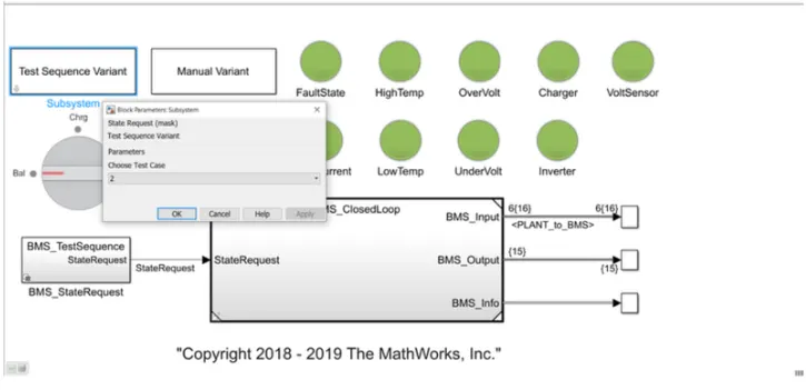
CASE:-2 Now change the test sequence varient in case two.

Sequence 2

Now by clicking on the BMS state request block

MODEL

From the above graph , a fault condition occured in second case. So even after charging was started, the soc didnt increase. It continue to decrease.

Simulation Result 2

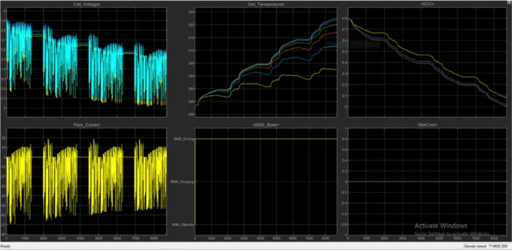
i) Driving Mode (0-10000 sec):- The cell voltage varies from 3.9 V to 3.05 volt ehich is cut off voltage of cell and the entire cell is drained upto 8692 sec.

Cell temperatures varies from 288K to 322.5K.

SOC reduces from 80% to 0% (cell got fully drained) in the drive mode under 8692 sec.

Cell balancing is not performed here.

ii) Charging Mode (10000- 20000 sec): The cell got drained earlier before reacching this mode.

CASE:- 3

Now by changing the test Sequence Value to 3

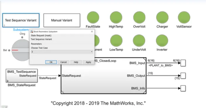
This condition has only one phase and that is charging.Thus 0 to 20000 seconds simulation runs

Sequence 3

Simulation Result 3

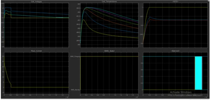
i) Charging (0-20000 sec):- Cell Voltages increases from there intial values and after 2000 sec they got constant .

Pack current initally start from 0 to 30A and then start decreasing when the constant voltage mode is there to 2.5 A and got full charged upto 2000 sec.

SOC was initally 80% and in 2000 sec it got fully charged that is 100%.

Cell temperature starts to incraeses initally and when battery got fully charged then decrease down to the ambient temperature.

Q2. What is coulomb counting? Refer to the above model and explain how BMS implements coulomb counting for SOC estimation ?

Ans2.

COULOMB COUNTING

Coulomb counting is a technique used to track the State of Charge of a battery pack. It works by integrating the active flowing current (measured in amps) over time to derive the total sum of energy entering or leaving the battery pack. SoC Estimation by Coulomb Counting is based on the measurement of the current and integration of that current over time. The State of Charge (SoC) of a battery cell is required to maintain it’s safe operation and lifetime during charge, discharge and storage. However, SoC cannot be measured directly and is estimated from other measurements and known parameters. This leads to errors in the estimated SoC and that means it is not possible to fully exploit the full capability of the cell. Coulomb counting gives a relative change in SoC and not an absolute SoC. If you measure the current over a given time step you have a measure of the number of Ah that have left or been received by the battery.

`SoC(t) = SOC(t-1)+I(t)/(Q(n))* Δt`

where:

• SoC(t) = estimated State of Charge at time, t
• SoC(t-1) = previous State of Charge at time t-1
• I(t) = charging or discharging current at time, t
• Q_n = battery cell capacity
• Δt = time step between t-1 and t

The BMS file that is given to us in the BMS project file is bellow

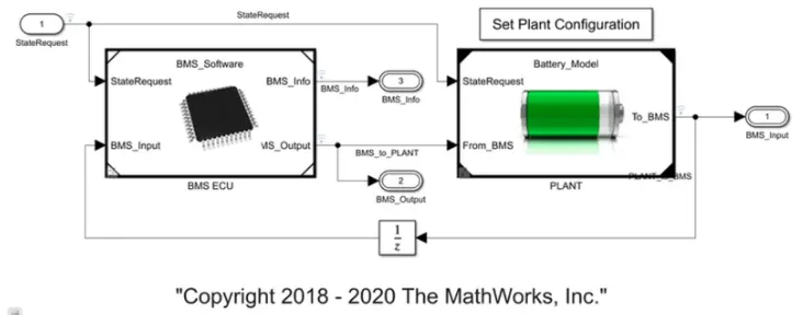
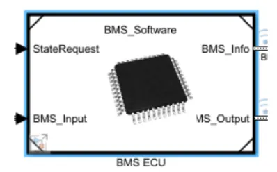
By Clicking on the BMS ECU we get the Subsystem

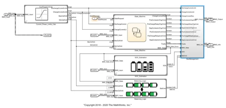
By clicking on the SOC estimation block we get

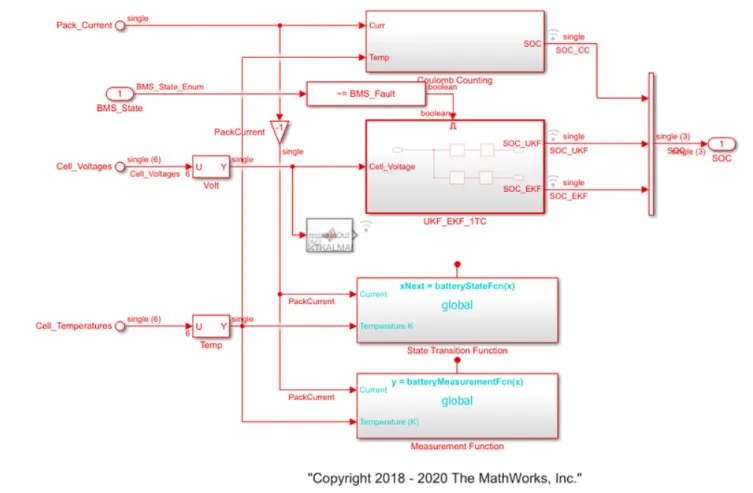
From above figure we select the Coulomb Counting block.

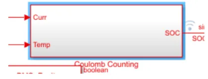
A subsystem opens when we click on the Coulomb Counting, this subsystem shows the logic used to calcutate the Coulomb Counting

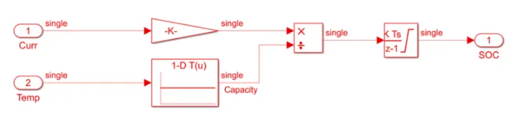
• This system does the estimation by coulomb counting equation mentioned above.
• Advantage of coulomb counting method is its simplicity and low computational cost.
• Temperature and current from the battery is given as inputs.
• Current signal is given to a gain block and temperature is given to capacity since it varies according to temperature.
• These inputs are given for integration where current will be integrated with respect to time.
• This outout is given to another block where it is divided by capacity.
• Hence the SOC is estimated.