Project 1 - Parsing NASA thermodynamic data
Aim:-
The aim of the project is to extract all 14 co-efficient from the NASA Thermodynamic Data for all 53 species and calculate the Specific Heat, Enthalpy, & Entropy for all the species and plot graph for them, and also calculates the molecular weight for all the species
Theory:-
NASA came up with polynomial that can be used to evaluate the thermodynamic properties such as Specific Heat, Enthalpy, & Entropy for more than 1000 species. They have also documented the co-efficient required to solve these polynomials. The polynomials are given bellow-
The co-efficient list contains 14 co-efficient for each species out which first 7 are high temperature co-efficient and last 7 are low temperature co-efficient, also local and global temperature range for all species.
Procedure:-
To start with we need to read the data been provided (Thermo.dat) so we us the ‘fgetl’ command to load the data and save in a variable ‘f1’ in read mode.
Now we extract the global temperatures from the second line and we skip the next 3 lines as they are just comments
Then to extract the local temperature ranges and coefficients we use the ‘for’ loop for all 53 species (we got to know about 53 species by looking at the data). First we identify the species name and then local temperatures by locating them in the particular line.
As we have extracted them as a string now we have to convert them to number so we use str2num command (but MATLAB suggested to use str2double for fast processing so str2double used).
In the same way we identify all the 14 coefficients and convert them into number.
And as the loop proceeds we get the value of coefficients for all 53 species.
Now to calculate the specific heat, enthalpy, entropy & molecular weight we have made function of each so we recall them in our main code within the ‘for’ loop as we need to do calculation for all 53 species.
Then to make plots of the specific heat, enthalpy, entropy we use the ‘plot’ command and label axes and give it a title and save the plot for each species by using ‘saveas’ command.
Now we need to save all the data in separate folder within the species folder so we use the ‘mkdir’ command to create the directory (folder) and use ‘cd’ command to enter the folder created and then again used ‘cd’ command to return to folder where our MATLAB program is present (as MATLAB program will only run when we are in the folder where program is present.
Main Code
close all
clear all
clc

%reading the NASA data file
f1 = fopen('THERMO.dat','r');
gt = fgetl(f1);
%reading the global temprature
global_temp = fgetl(f1);
x = strsplit(global_temp,' ');
global_low_temp = str2num(x{2});
global_mid_temp = str2num(x{3});
global_high_temp = str2num(x{4});

%skipping next 3 lines
fgetl(f1);
fgetl(f1);
fgetl(f1);

%universal gas constant
R = 8.314;

% as we know data file contains 53 species so we make as for loop for 53
% iterations

for i = 1:53
    line1 = fgetl(f1);
    a = strsplit(line1,' ');
    species = (a{1});
    % finding the local temprature range
    b = strfind(line1,'G');
    local_low_temp = line1(b+3:b+10);
    local_high_temp = line1(b+13:b+20);
    local_mid_temp = line1(b+23:b+30);
    l_t = str2double(local_low_temp);
    m_t = str2double(local_mid_temp);
    h_t = str2double(local_high_temp);

    %reading coefficient data from line 1
    line2 = fgetl(f1);
    p = strfind(line2,'E');
    c1 = line2(1:p(1)+3);
    c1 = str2num(c1);
    c2 = line2(p(1)+4:p(2)+3);
    c2 = str2num(c2);
    c3 = line2(p(2)+4:p(3)+3);
    c3 = str2num(c3);
    c4 = line2(p(3)+4:p(4)+3);
    c4 = str2num(c4);
    c5 = line2(p(4)+4:p(5)+3);
    c5 = str2num(c5);

    %reading coefficient data from line 2
    line3 = fgetl(f1);
    q = strfind(line3,'E');
    c6 = line3(1:q(1)+3);
    c6 = str2num(c6);
    c7 = line3(q(1)+4:q(2)+3);
    c7 = str2num(c7);
    c8 = line3(q(2)+4:q(3)+3);
    c8 = str2num(c8);
    c9 = line3(q(3)+4:q(4)+3);
    c9 = str2num(c9);
    c10 = line3(q(4)+4:q(5)+3);
    c10 = str2num(c10);

    %reading coefficient data from line 3
    line4 = fgetl(f1);
    r = strfind(line4,'E');
    c11 = line4(1:r(1)+3);
    c11 = str2num(c11);
    c12 = line4(r(1)+4:r(2)+3);
    c12 = str2num(c12);
    c13 = line4(r(2)+4:r(3)+3);
    c13 = str2num(c13);
    c14 = line3(r(3)+4:r(4)+3);
    c14 = str2num(c14);

    %taking 100 local tempratures between local low temp and local high temp

    t = linspace(l_t, h_t, 100);

    % calculating specific heat Cp

    Cp = specific_heat(c1,c2,c3,c4,c5,c8,c9,c10,c11,c12,t,R, m_t);

    % calculating enthalpy H
    H = enthalpy(c1,c2,c3,c4,c5,c6,c8,c9,c10,c11,c12,c13,t,R,m_t);

    % calculating entropy S
    S = entropy(c1,c2,c3,c4,c5,c7,c8,c9,c10,c11,c12,c14,t,R,m_t);

    % calculating molecular weight m_wt
    m_wt = molecular_weight(species);
    m_wt_file = fopen('molecular_weight.text','a+');
    fprintf(m_wt_file,'The Moleculare weight of %s is %d n',species,m_wt );
    fclose(m_wt_file);


    % saving as a folder
    cur_dir = pwd;
    mkdir(species);
    cd(species);

    %ploting Cp vs T
    figure(1)
    plot(t,Cp,'LineWidth',2,'Color','r');
    xlabel('temprature')
    ylabel('specific heat')
    title('Specific heat vs temprature')

    % Ploting H vs T
    figure(2)
    plot(t,H,'LineWidth',2,'Color','r');
    xlabel('temprature')
    ylabel('Enthalpy')
    title('Enthalpy vs temprature')

    %Ploting S vs T
    figure(3)
    plot(t,S,'LineWidth',2,'Color','r');
    xlabel('temprature')
    ylabel('Entropy')
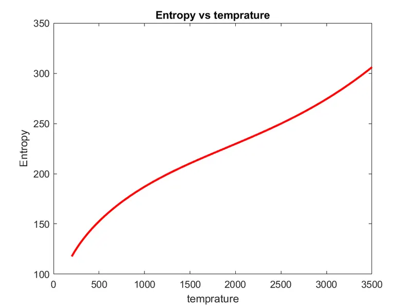
    title('Entropy vs temprature')

    saveas(figure(1),'Specific_heat.png')
    saveas(figure(2),'Enthalpy.png')
    saveas(figure(3),'Entropy.png')

    cd(cur_dir);

end
Function Code:-
Specific Heat:-
For specific heat we have polynomial as
So as we have 2 sets of coefficients (1 for high temperature and other for low temperature), so we use the ‘if else’ command for this case
If temperature is greater than mid temperature than we use the first 7 coefficients else we use other 7 coefficients
Function for Specific Heat
function Cp = specific_heat(c1,c2,c3,c4,c5,c8,c9,c10,c11,c12,t,R,m_t)
if t>m_t
    Cp = (c1+c2.*(t)+c3.*(t.^2)+c4.*(t.^3)+c5.*(t.^4)).*R;
else
    Cp = (c8+c9.*(t)+c10.*(t.^2)+c11.*(t.^3)+c12.*(t.^4)).*R;
end
end
Enthalpy:-
For enthalpy we have polynomial as
So as we have 2 sets of coefficients (1 for high temperature and other for low temperature), so we use the ‘if else’ command for this case
If temperature is greater than mid temperature than we use the first 7 coefficients else we use other 7 coefficients
Function for Enthalpy
function H = enthalpy(c1,c2,c3,c4,c5,c6,c8,c9,c10,c11,c12,c13,t,R,m_t)
if t>m_t
    H = (c1+c2.*(t./2)+c3.*(t.^2)./3+c4.*(t.^3)./4+c5.*(t.^4)./5+c6./t).*t.*R;
else
    H = (c8+c9.*(t./2)+c10.*(t.^2)./3+c11.*(t.^3)./4+c12.*(t.^4)./5+c13./t).*t.*R;
end
end
Entropy:-
For specific heat we have polynomial as
So as we have 2 sets of coefficients (1 for high temperature and other for low temperature), so we use the ‘if else’ command for this case
If temperature is greater than mid temperature than we use the first 7 coefficients else we use other 7 coefficients
Function for Entropy
function S = entropy(c1,c2,c3,c4,c5,c7,c8,c9,c10,c11,c12,c14,t,R,m_t)
if t>m_t
    S = R*((c1.*(log(t)))+(c2.*t)+(c3.*(t.^2)/2)+(c4.*(t.^3)/3)+(c5.*(t.^4)/4)+c7);
else
    S = R*((c8.*(log(t))+(c9.*t)+(c10.*(t.^2)/2)+(c11.*(t.^3)/3)+(c12.*(t.^4)/4))+c14);
end
end
Molecular Weight:-
For calculation of molecular weight we provide the molecular weight of some basic elements, then with the help of these elements we calculate the molecular weight for all the species
For this we use the ‘for’ loop with the length of the number of species and second ‘for’ loop with the length of provided number of atomic wt and then we use if loop to compare the species name with the given atomic name and calculate the molecular weight accordingly
Now to display the molecular weight in the command window we use ‘fprintf’ command
Function for Calculation of Molecular Wt
function m_wt = molecular_weight(species)
atomic_name = ['H', 'C', 'N', 'O', 'AR'];
atomic_wt = [1.008 12.011 14.007 15.999 39.948];
m_wt=0;
for i = 1:length(species)
    for j = 1:length(atomic_wt)
        if strcmpi(species(i),atomic_name(j))
            m_wt=m_wt+atomic_wt(j);
            position = j;
        end
    end
    n = str2num(species(i));
    if n>1
        m_wt = m_wt+atomic_wt(position)*(n-1);
    end
end
fprintf('molecular_weight of %s :-',species);
fprintf('%f',m_wt);
disp(':');
end
Conclusion :-
As the result we get the folders named after species and containing the plots for Specific Heat, Enthalpy & entropy and also we get the molecular weight displayed on the command window and also saved as a text file
Screen Shot of the folder containing the sub folder of all the species

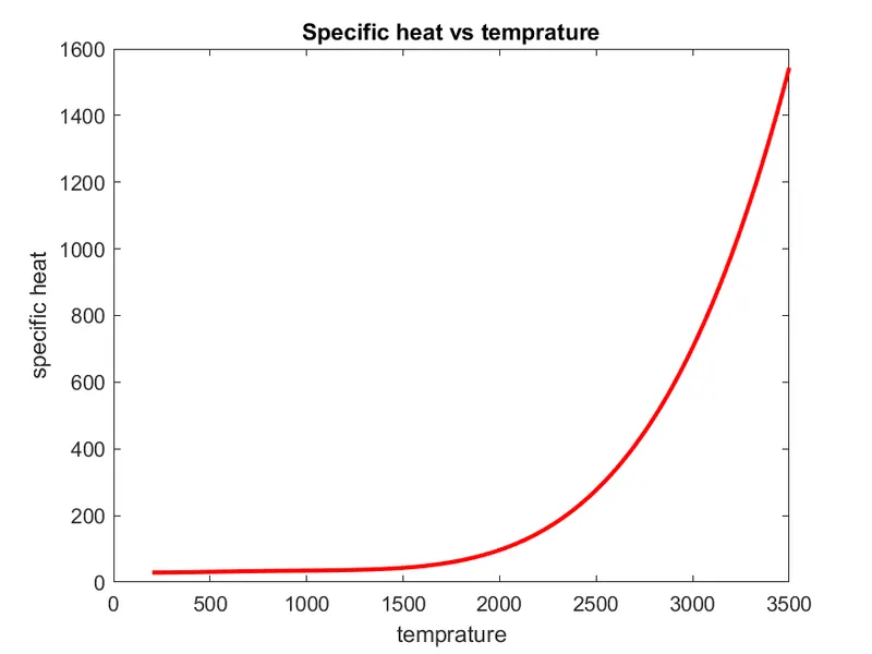
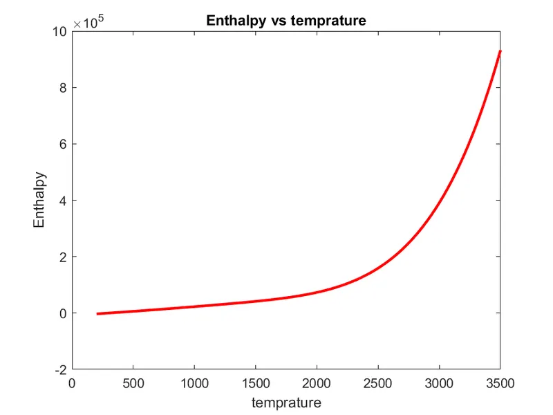
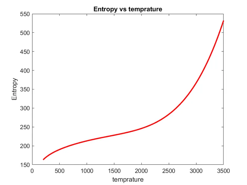
Plots for the result of O2
Specific Heat vs Temprature
Enthalpy vs Temprature
Entropy vs Temprature
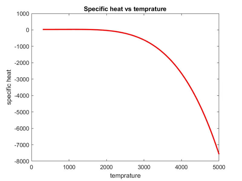
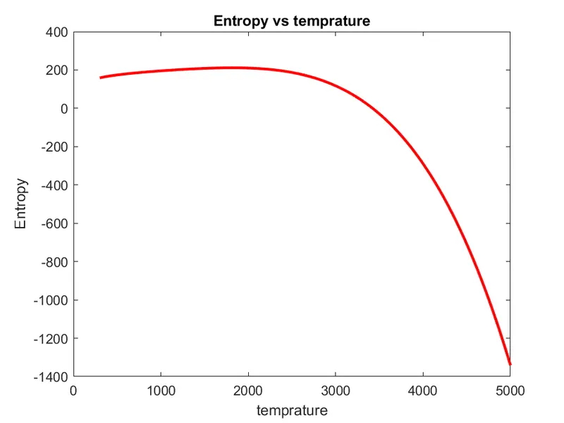
Plots for the result of N2
Specific Heat vs Temprature
Enthalpy vs Temprature
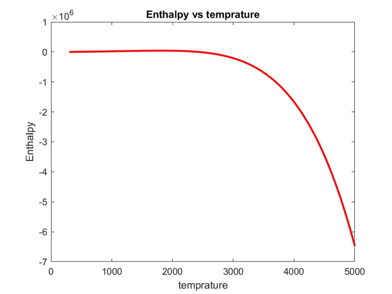
Entropy vs Temprature
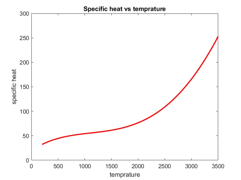
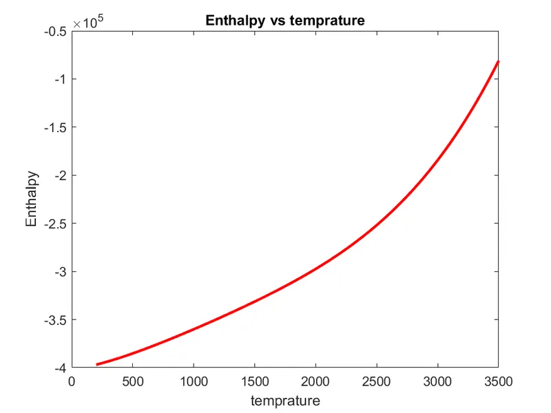
Plots for the result of CO2
Specific Heat vs Temprature
Enthalpy vs Temprature
Entropy vs Temprature
Molecular Weight of all Species as shown in command window
molecular_weight of O :-15.999000:
molecular_weight of O2 :-31.998000:
molecular_weight of H :-1.008000:
molecular_weight of H2 :-2.016000:
molecular_weight of OH :-17.007000:
molecular_weight of H2O :-18.015000:
molecular_weight of HO2 :-33.006000:
molecular_weight of H2O2 :-34.014000:
molecular_weight of C :-12.011000:
molecular_weight of CH :-13.019000:
molecular_weight of CH2 :-14.027000:
molecular_weight of CH2(S) :-14.027000:
molecular_weight of CH3 :-15.035000:
molecular_weight of CH4 :-16.043000:
molecular_weight of CO :-28.010000:
molecular_weight of CO2 :-44.009000:
molecular_weight of HCO :-29.018000:
molecular_weight of CH2O :-30.026000:
molecular_weight of CH2OH :-31.034000:
molecular_weight of CH3O :-31.034000:
molecular_weight of CH3OH :-32.042000:
molecular_weight of C2H :-25.030000:
molecular_weight of C2H2 :-26.038000:
molecular_weight of C2H3 :-27.046000:
molecular_weight of C2H4 :-28.054000:
molecular_weight of C2H5 :-29.062000:
molecular_weight of C2H6 :-30.070000:
molecular_weight of CH2CO :-42.037000:
molecular_weight of HCCO :-41.029000:
molecular_weight of HCCOH :-42.037000:
molecular_weight of H2CN :-28.034000:
molecular_weight of HCN :-27.026000:
molecular_weight of HNO :-31.014000:
molecular_weight of N :-14.007000:
molecular_weight of NNH :-29.022000:
molecular_weight of N2O :-44.013000:
molecular_weight of NH :-15.015000:
molecular_weight of NH2 :-16.023000:
molecular_weight of NH3 :-17.031000:
molecular_weight of NO :-30.006000:
molecular_weight of NO2 :-46.005000:
molecular_weight of HCNO :-43.025000:
molecular_weight of HOCN :-43.025000:
molecular_weight of HNCO :-43.025000:
molecular_weight of NCO :-42.017000:
molecular_weight of CN :-26.018000:
molecular_weight of HCNN :-41.033000:
molecular_weight of N2 :-28.014000:
molecular_weight of AR :-39.948000:
molecular_weight of C3H8 :-44.097000:
molecular_weight of C3H7 :-43.089000:
molecular_weight of CH3CHO :-44.053000:
molecular_weight of CH2CHO :-43.045000:
ERRORS:-
Error 1:-
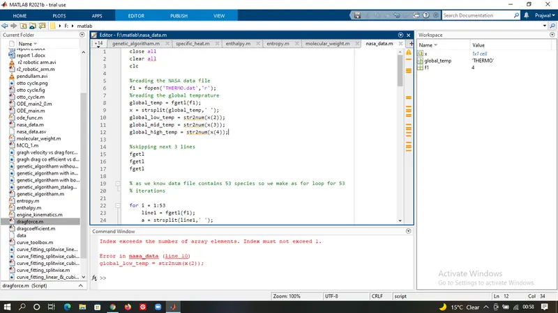
In above image issue was the data was not present the line so we need to skip first line of header as it was title of the file does not contain any ' '.
to resolve title line of header was skipped(added line gt = fgetl(f1))
Error 2 :-
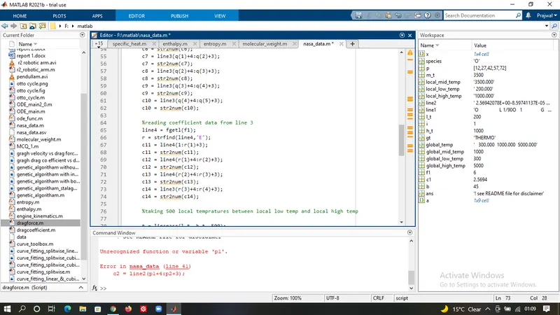
The issue in above image is a typing error instead of p(1) p1 was used
Error 3:-
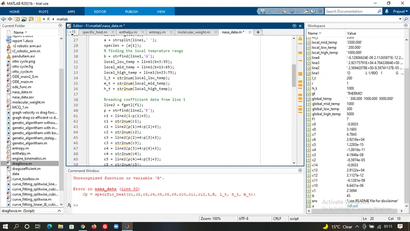
The error in above image is the variable R was not defined, to resolve R was given the value of 8.314(universal gas constant)
Error 4:-
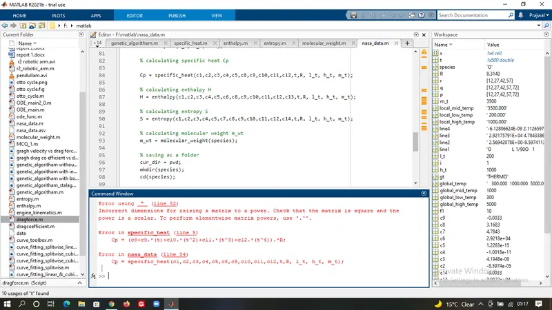
The error in above image is the element wise operator was not used in the equation, to resolve element wise operator was used.