PV Diagram of the Otto cycle

Report:-

Aim: - To plot the PV Diagram for the otto cycle

Procedure: -

To plot the PV diagram of the otto cycle, we require volume (v) and pressure (p) at all the 4 stages of the otto cycle (compression, ignition, expansion, exhaust)

Geometric parameters of the engines are provided

bore:- 0.1

stroke:- 0.1

connecting rod (con_rod):- 0.15

compression ratio(cr)=12

So to calculate state variables at state point 1

swept volume(v_swept) = (pi/4)*bore^2*stroke

clearance volume(v_clearance) = v_swept/(cr-1);

v1 = swept volume + clearance volume

p1 = 101325 (provided)

t1 = 500 (provided)

So to calculate state variables at state point 2

v2 = v_clearance;

p2v2^gamma = p1v1^gamma (p1v1^gamma=p2v2^gamma)

p2 = p1*(v1/v2)^gamma (v1/v2 = cr)

p2 = p1*cr^gamma

t2 = p2*v2*t1/ (p1*v1) (p1v1/t1=p2v2/t2)

So to calculate state variables at state point 3

v3=v2

p3 = p2*(t3/t2) (p3v3/t3 = p2v2/t2)

t3 = 2300 (provided)

So to calculate state variables at state point 4

v4 = v1

p4 = p3*(v3/v4)^gamma (p3v3^gamma = p4v4^gamma)

So, now to plot the all the 4 state variables we use ‘plot’ command, with ‘hold on’ command otherwise we will get 4 plot but we required all the 4 plots on one figure so we use ‘hold on’ command

plot(v1,p1,'*', 'color','r');

plot(v2,p2,'*', 'color','r');

plot(v3,p3,'*', 'color','r');

plot(v4,p4,'*', 'color','r');

with these command we will get the point of all the state variables but now we need to connect these points according to our requirement(we need a curve line to represent isentropic compression and expansion)

So for this we need to calculate how the volume changes inside the combustion cylinder so

v = 1+{0.5*(cr-1)}*[{r+1-cosd(theta)}-{(r^2-sind(theta).^2).^0.5}].(v_clearance)

now to simplify we divide this equation into 3 terms

term1 = 0.5*(cr-1)

term2 = r+1-cosd(theta)

term3 = (r^2-sind(theta).^2).^0.5

for above equation theta varies from start crank angle to end crank angle with 100 values in between them so we use

theta=linspace(start_crank, end_crank,100);

Now all these calculation for volume can be used as a function[v] so that we can recall the function when we require in our main program

With the help of above function we can calculate the compression volume and expansion volume

For compression volume:-

constant_c= p1*v1^gamma;

v_compression = engine_kinematics(bore, stroke, con_rod, cr, 180, 0);

p_compression = constant_c./v_compression.^gamma;

For expansion volume:-

constant_c= p3*v3^gamma;

v_expansion = engine_kinematics(bore, stroke, con_rod, cr, 0, 180);

p_expansion = constant_c./v_expansion.^gamma;

(In the above expression we have to use an element-wise operator to multiply the matrix with the single element)

Now we have calculate our all the required input and we have already plotted the points of all the state variable now we can join them by following codes

plot(v_compression, p_compression);

plot([v2 v3],[p2 p3], 'color','b');

plot(v_expansion, p_expansion);

plot([v4 v1],[p4 p1], 'color','b');

Now we have to calculate the thermal efficiency of the engine, which is

efficiency = [(1- (t1/t2)]*100

Main Code:-

% Otto cycle

clear all
close all
clc

% inputs
gamma = 1.4;
t3 = 2300;

% state varaible at state point 1
p1 = 101325;
t1 = 500;

% engine geometric parameters
bore = 0.1;
stroke = 0.1;
con_rod = 0.15;
cr = 12;

% calculation the swept volume & clearance volume
v_swept = (pi/4)*bore^2*stroke;
v_clearance = v_swept/(cr-1);

v1 = v_swept + v_clearance;
v2 = v_clearance;

% state varaible at state point 2
% p2v2^gama = p1v1^gamma
% p2 = p1*(v1/v2)^gamma
% v1/v2 = cr
% p2 = p1*cr^gamma
p2 = p1*cr^gamma;

% p1v1/t1=p2v2/t2
% t2 = p2v2t1/(p1v1)
t2 = p2*v2*t1/(p1*v1);

constant_c= p1*v1^gamma;
v_compression = engine_kinematics(bore, stroke, con_rod, cr, 180, 0);
p_compression = constant_c./v_compression.^gamma;


% state variable at state point 3
v3 = v2;

% p3v3/t3 = p2v2/t2
% p3 = p2(t3/t2)
p3 = p2*(t3/t2);
constant_c= p3*v3^gamma;
v_expansion = engine_kinematics(bore, stroke, con_rod, cr, 0, 180);
p_expansion = constant_c./v_expansion.^gamma;


% state variable at state point 4
v4 = v1;        

% p3v3^gamma = p4v4^gamma
% p4 = p3(v3/v4)^gamma
p4 = p3*(v3/v4)^gamma;

figure(1)
hold on
plot(v1,p1,'*', 'color','r');
plot(v_compression, p_compression);
plot(v2,p2,'*', 'color','r');
plot([v2 v3],[p2 p3], 'color','b');
plot(v3,p3,'*', 'color','r');
plot(v_expansion, p_expansion);
plot(v4,p4,'*', 'color','r');
plot([v4 v1],[p4 p1], 'color','b');

% thermal efficiency of the engine

efficiency = [1 - (t1/t2)]*100;

Function code:-

%engine kinematics
function [V] = engine_kinematics(bore, stroke, con_rod, cr, start_crank, end_crank)

a = stroke/2;
r = con_rod/a;

v_s = pi/4*bore^2*stroke;
v_c = v_s/(cr-1);

theta=linspace(start_crank, end_crank,100);

term1 = 0.5*(cr-1);
term2 = r+1-cosd(theta);
term3 = (r^2-sind(theta).^2).^0.5;

V = (1+term1*(term2-term3)).*v_c;

end

Conclusion:-

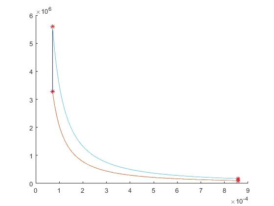
As the result of the function, we get the array of 100 values each for compression volume and expansion volume and with the help of these values we are able to plot the PV Diagram of the otto cycle & the thermal efficiency of the engine(62.9893%)

Result of the code

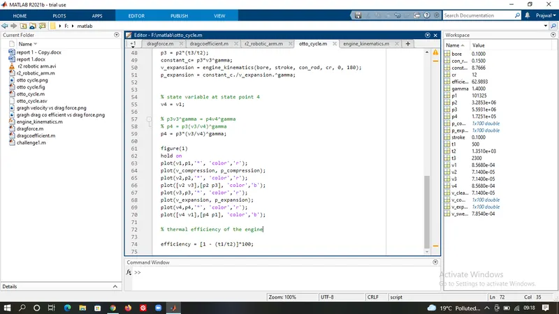
The plot of the code

Error faced during compilation

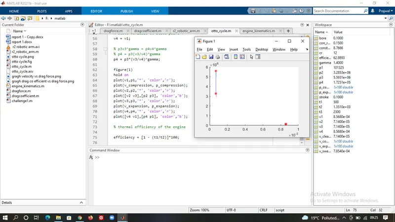
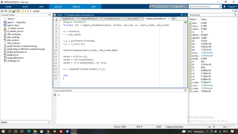
the issue in the above image was that the graph plotted was not as expected, so after checking it was found that there was a typing mistake in the function code in the formula

in term 1 (/) was used instead of (*), due to which all the values were calculated but the value for changing volume was incorrect due to which graph was not plotted properly