Week 4.1 - Genetic Algorithm
Aim:-
The aim of the project is to find the global maxima using stalagmite function in genetic algorithm.
Theory:-
Genetic algorithm is the most commonly used optimization tool. It is based on the Darwin’s theory of natural selection. In genetic algorithm we use the current population as the parent population and then we make their crossover and mutate them over the time to get optimum solution.
In MATLAB, the genetic algorithm function in the inbuilt command that gives us the global minima of the function, so in-order to get the global maxima we need to invert the function (i.e. the negative value of the function will give the maximum value of the function.
Syntax of the Genetic Algorithm in MATLAB
According to our requirement we can use the syntax of GA as following
x = ga(fun,nvars)
x = ga(fun,nvars,A,b)
x = ga(fun,nvars,A,b,Aeq,beq)
x = ga(fun,nvars,A,b,Aeq,beq,lb,ub)
x = ga(fun,nvars,A,b,Aeq,beq,lb,ub,nonlcon)
x = ga(fun,nvars,A,b,Aeq,beq,lb,ub,nonlcon,options)
x = ga(fun,nvars,A,b,Aeq,beq,lb,ub,nonlcon,intcon)
x = ga(fun,nvars,A,b,Aeq,beq,lb,ub,nonlcon,intcon,options)
where,
fun — function handle/name
nvars — Number of variables
A — Linear inequality constraints
Aeq — Linear equality constraints
b — Linear inequality constraints
beq — Linear equality constraints
lb — Lower bounds
ub — Upper bounds
nonlcon — Nonlinear constraint
options — Optimization options
intcon — Integer variables
Note:- for no value of A,b,Aeq,beq,lb,ub,nonlcon,intcon use ‘[]’
Procedure:-
To start with we use the ‘linspace’ command to create the vector matrix of x & y and the create a 2D array with the help of ‘meshgrid’ command and we take the number of iteration to be 50.
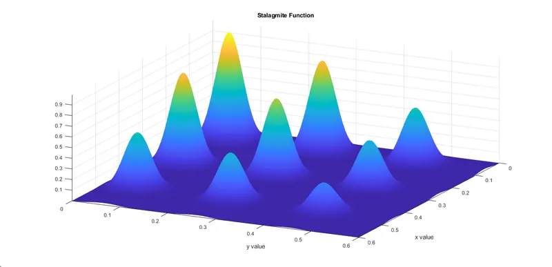
Now to create the plot for the stalagmite function we use the nested for loop with i & j as the loop counter for each loop and then we recall our stalagmite function that we have already created by using the formula
Now, plot the surface plot for (xx, yy, -f)
(Used (–f) as we need to get the maximum value but the function gives the minimum value)
Enable shading interp in order to make the plot look smooth, and label the axis and give title to the plot
- Case 1 (for no boundary conditions)
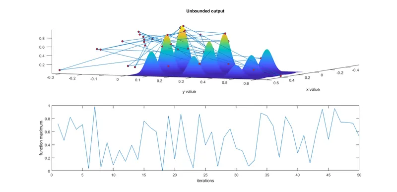
To calculate the optimal result for the unbounded condition we use the GA command in the ‘for’ loop with the syntax
x = ga(fun,nvars)
and we use the tic-toc command to calculate time taken for optimization.
In this for loop every value for the result is saved in xopt, yopt and fopt variables and we make the plot out of these variables and plot 1 more graph for (-fopt)
- Case 2 (for boundary conditions (0~0.6)
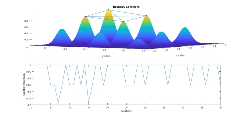
To calculate the optimal result for the boundary condition we use the GA command in the for loop with the syntax
x = ga(fun,nvars,A,b,Aeq,beq,lb,ub)
and in place of A,b,Aeq,beq use [] and lb as [0,0] and ub as [0.6,0.6]
and we use the tic-toc command to calculate time taken for optimization.
In this for loop every value for the result is saved in xopt, yopt and fopt variables and we make the plot out of these variables and plot 1 more graph for (-fopt)
- Case 3 (fro boundary condition with increased population)
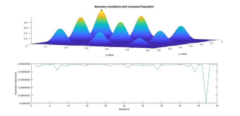
To calculate the optimal result for the boundary condition with increased population we use the GA command in the for loop with the syntax
x = ga(fun,nvars,A,b,Aeq,beq,lb,ub,nonlcon,intcon,options)
and in place of A,b,Aeq,beq,nonlcon,intcon use [] and lb as [0,0] and ub as [0.6,0.6]
and in option we increase the population to 1000 by using the command
options = optimoptions(@ga,'populationSize',1000)
and we use the tic-toc command to calculate time taken for optimization.
In this for loop every value for the result is saved in xopt, yopt and fopt variables and we make the plot out of these variables and plot 1 more graph for (-fopt)
Function Code
function [f] = stalagmite(input_vector)
x = input_vector(1);
y = input_vector(2);

f1_x = (sin(5.1*pi*x + 0.5)).^6;
f1_y = (sin(5.1*pi*y + 0.5)).^6;

term1 = ((x-0.0667)^2)/(0.64);
f2_x = exp(-4.*log(2)*term1);

term2 = ((y-0.0667)^2)/(0.64);
f2_y = exp(-4.*log(2)*term2);

f = -(f1_x.*f2_x.*f1_y.*f2_y);

end
Main Code
close all
clear all
clc

% independent variables
x = linspace(0, 0.6, 150);
y = linspace(0, 0.6, 150);

% creating  2d array
[xx, yy] = meshgrid(x,y);

% No of iterations
num_case = 50;

% creating the surface plot for stalagmite function by nested for loop

for i=1:length(x)
    for j=1:length(y)
        input_vector(1) = xx(i,j);
        input_vector(2) = yy(i,j);
        f(i, j) = stalagmite(input_vector);
    end
end

% creating the 3-D surface plot

figure(1)
surfc(xx, yy,-f)

% to make plot look smoother use shading interp
shading interp
xlabel('x value')
ylabel('y value')
title('Stalagmite Function')

% case study 1(unbounded)
%to calculate time taken for optimization use tic toc command
tic
for i = 1:num_case
    [input, fopt(i)] = ga(@stalagmite,2);
    xopt(i) = input(1);
    yopt(i) = input(2);
end
case_time_1=toc
figure(2)
subplot(2,1,1)

hold on
surfc(xx,yy,-f)

xlabel('x value')
ylabel('y value')
title('Unbounded output')
shading interp
hold on
plot3(xopt,yopt,-fopt,'marker','o','MarkerSize',5,'MarkerFaceColor','r')
subplot(2,1,2)
plot(-fopt)
xlabel('iterations')
ylabel('function maximum')

% case study 2(with upper and lower boundary conditions
tic
for i = 1:num_case
    [input, fopt(i)] = ga(@stalagmite,2,[],[],[],[],[0;0],[0.6;0.6]);
    xopt(i) = input(1);
    yopt(i) = input(2);
end
case_time_2=toc
figure(3)
subplot(2,1,1)

hold on
surfc(xx,yy,-f)

xlabel('x value')
ylabel('y value')
title('Boundary Conditions')
shading interp
hold on
plot3(xopt,yopt,-fopt,'marker','o','MarkerSize',5,'MarkerFaceColor','r')
subplot(2,1,2)
plot(-fopt)
xlabel('iterations')
ylabel('fucnction maximum')

% case study 3(increase the polulation)
options = optimoptions(@ga)
options = optimoptions(@ga,'populationSize',1000)

tic
for i = 1:num_case
    [input, fopt(i)] = ga(@stalagmite,2,[],[],[],[],[0;0],[0.6;0.6],[],[],options);
    xopt(i) = input(1);
    yopt(i) = input(2);
end
case_time_3=toc
figure(4)
subplot(2,1,1)

hold on
surfc(xx,yy,-f)

xlabel('x value')
ylabel('y value')
title('Boundary comditions with increased Population')
shading interp
hold on
plot3(xopt,yopt,-fopt,'marker','o','MarkerSize',5,'MarkerFaceColor','r')
subplot(2,1,2)
plot(-fopt)
xlabel('iterations')
ylabel('fucnction maximum')
Plot 1
Plot 2
Plot 3
Plot 4
Conclusion:-
We can see that as the unbounded plot shows the values beyond the desired limit of (0~0.6) and we get the scattered plot as we apply the boundary limits the values came between the required limits and the plot gets more localized and as we increase the size of the population the plot gets more concentrated and we get the global maxima
As we increase the bounds and population the time taken for optimization increases.
Errors During Compilation
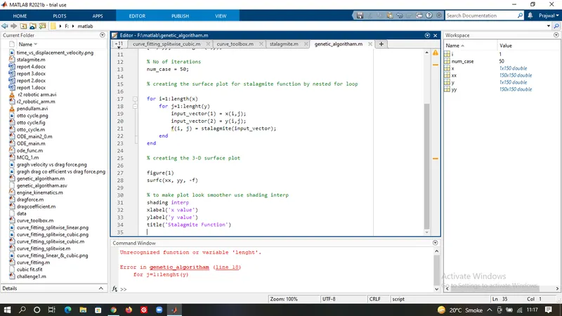
Typing Error in length Command
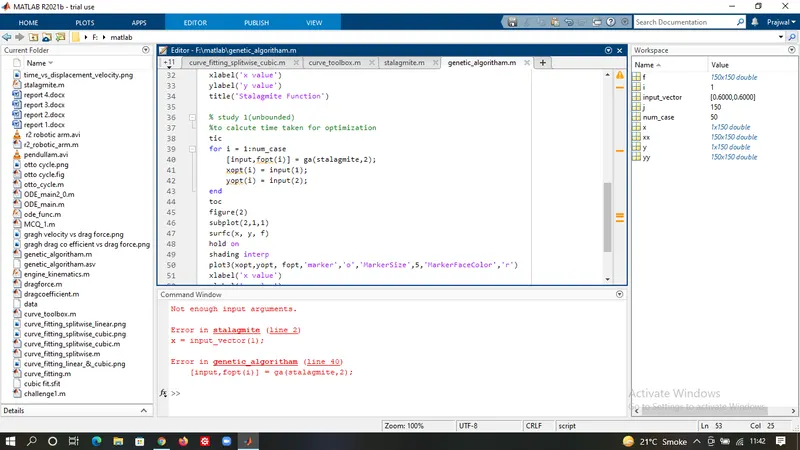
Error in GA syntex '@' Not used
Referances
1. https://en.wikipedia.org/wiki/Genetic_algorithm
2. https://in.mathworks.com/help/gads/genetic-algorithm.html