Week 3 - Solving second order ODEs
Aim:
The aim of the project is to create the animation of the pendulum whose governing equation is 2nd order differential equation.
Procedure:-
To make the animation of the pendulum we need to solve the 2nd order Differential equation by which the motion of the pendulum is govern.
The provided inputs are:-
g = gravity in m/s2 (g=9.81 m/s)
L = length of the pendulum in m (L=1 meter)
m = mass of the ball in kg (m=1 kg)
b=damping coefficient (b=0.05)
Time Span = 0~20(with 500 frames in between)
Initial Angular velocity = 3rad/sec
The Equation by which the motion is govern is:-
Now to get the velocity and displacement we need to solve this differential equation, so now in order to solve this equation we need to reduce 2nd order Differential equation to 1st order Differential equation and then make it a function and then we need to call the function when we use the 'ode45' inbuilt ODE solver of MATLAB, for this solver to work we need to provide the data of differential equation in matrix form
So in order to reduce 2nd order Differential equation to 1st order Differential equation we create a function which takes t, theta, b, g, l, m, as input so now
theta1 = theta(1)
theta2 = theta(2)
dtheta1_dt = theta2
dtheta2_dt = [-(b/m)*theta2]-[(g/l)*sin(theta1)]
dtheta_dt = (dtheta1_dt; dtheta2_dt)
now this function is saved by the name ode_func
so now to solve this equation we use the ode45 code
[t, result] = ode45(@(t, theta) ode_func(t, theta, b, g, l, m), t_span, theta_0)
Our ODE is the function of t and theta and then we define our ODE function (ode_func) than we provide time span and then we give the initial condition. As this solver takes and gives data in matrix form so we will have solution matrix in which we will get value of time wrto displacement & velocity(in result matrix which is of size 2x500)
Now as the result of this code we get the value of time, velocity and displacement
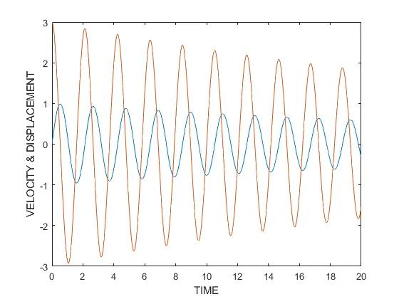
Now to plot the time vs. velocity & displacement graph we use plot command with hold on and hold off command and will save the graph in Figure 1(hold on and off command are used to use plot command multiple time without over writing the previous outcome of the plot)
figure(1)
plot(t, result(:,1));
hold on
plot(t, result(:,2));
hold off
xlabel('time)
ylabel('velocity & displacement')
Now in order to create the animation we use the 'for' loop with 'i' as loop counter and for every loop we increase the counter by 1 till the loop ends.so the code of this is
theta3 = result(:,1) (theta3 is the variable for displacement vector)
ct=1
for i=(1:length(theta3) (i will increase till the length of theta3 i.e. 500)
d=theta3(i) (for every loop new value of theta3 will be saved in d)
x0 = 0 (coordinates of pivot point)
y0 = 0
x1 = 1*cos(d) (coordinates of bob)
y1=-1*sin(d)
plot([-1 1], [ 0 0], 'linewidth',5,'color','m') (to plot the base line of the pendulum)
hold on
plot(x0,y0,'o', 'markerfacecolor','r') (to plot the pivot point)
plot([x0 x1],[y0 y1], 'linewidth',3,'color','b') (to plot the mass less string of the pendulum)
hold off
axis( -2 2 -2 2) (define the axis)
pause(0.02) (pause the frame to capture the frame)
M(ct)=getframe(gcf) (save frame of every loop in M)
ct = ct+1; (increase the counter by 1 in every loop)
end
Now to convert the saved frame into movie we use 'movie' command, to save it as a video file we have to give it a name, format & resolution in which it will be saved with the following commands
movie(M)
Videofile = Videowriter('pendulum.avi', 'uncompressed AVI')
open(videofile)
writevideo(videofile,M)
close(videofile)
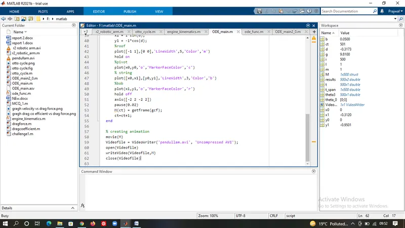
Main Code:-
clear all
close all
clc

%inputs
b=0.05;
g=9.81;
l=1;
m=1;

%initial conditions
theta_0=[0;3];

%timme points
t_span = linspace(0,20,500);

% solve ODE
[t, results] = ode45(@(t, theta) ode_func(t, theta, b, g, l, m), t_span,theta_0);
% plot for time vs velocity & displacement
figure(1)
plot(t, results(:,1));
hold on
plot(t, results(:, 2))
hold off
ylabel('VELOCITY & DISPLACEMENT')
xlabel('TIME')

figure(2)
theta3 = results(:,l);
ct = 1;

for i=1:length(theta3)
    d=theta3(i);

    % coordinates
    x0 = 0;
    y0 = 0;

    x1 = l*sin(d);
    y1 = -1*cos(d);
    %roof
    plot([-1 1],[0 0],'LineWidth',5,'Color','m')
    hold on
    %pivot
    plot(x0,y0,'o','MarkerFaceColor','c')
    % string
    plot([x0,x1],[y0,y1],'LineWidth',3,'Color','b')
    %bob
    plot(x1,y1,'o','MarkerFaceColor','r')
    hold off
    axis([-2 2 -2 2])
    pause(0.02)
    M(ct) = getframe(gcf);
    ct=ct+1;
end

% creating animation
movie(M)
Videofile = VideoWriter('pendullam.avi', 'Uncompressed AVI');
open(Videofile)
writeVideo(Videofile,M)
close(Videofile)
Function code:-
function [dtheta_dt] = ode_func(t, theta, b, g, l, m)

theta1 = theta(1);
theta2 = theta(2);
dtheta1_dt = theta2;
dtheta2_dt = -(b/m)*theta2 - (g/l)*sin(theta1);
dtheta_dt = [dtheta1_dt; dtheta2_dt];
end
Conclusion:-
With the help of above code we are able to create the animation for the pendulum by solving the second order differential equation using the ode45.
Result of the code
Plot of time vs displacement & velocity
Animation of the pendullam
Error Faced During Code compilaiton
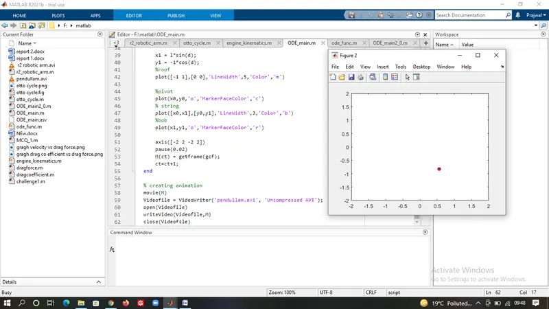
The issue in the above image is, hold command was not used so only last plot command was executed and rest plot commands were overwritten
After adding Hold on & Hold off command the issue was resolved