Week 7 State of charge estimation
The closed loop BMS control can be downloaded from the file exchange window at matworks.com using the given link.
After extracting the zip file we can access the closed loop BMS control model through MATLAB by accesing the Tests folder > System > BMS_closed_loop_Harness_dashboard model. The model file opens as:
Dashboard:
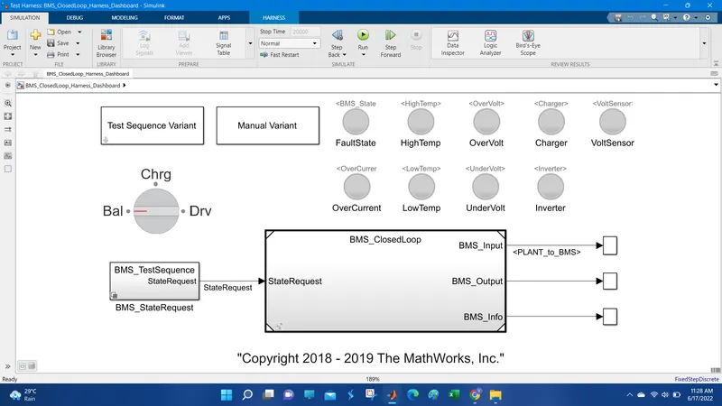
The Test cases are varied using the 'Test sequence variant block' in the model. The model also has a manual variant block to manually vary the selector. it also contains:
- BMS_testsequence state request which provides the state request commands.
- Lamps indicating fault state, overvoltage, High temperature, Charger, Voltage sensor, Over current, Low Temperature, Undervoltage, and inverter. Lamps turning red indicates fault has occured and green indicates all systems are working smoothly.
- Rotating switch for manual variant selector which has 3 modes: Balanced, Charging and Driving modes.
- The Scope shows the SOC of the module, Current of the module, cell voltages, cell temperature, battery state and cell balancing states.
BMS Closed Loop Model:
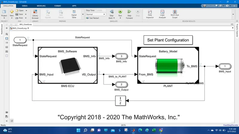
The state request from the dashboard is applied as input for the BMS closed loop model. It mainly consists of two components, the Plant and the BMS ECU. Plant is actually the battery model and the ECU provides the input for the plant. The plant output is fed back to the BMS ECU which acts as a feedback signal.
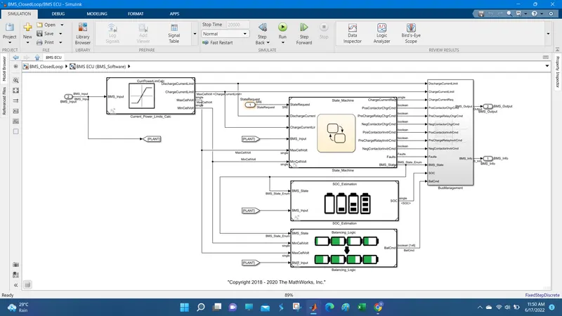
The above figure shows the BMS ECU subsystem. The Current power limit calculations block provides the discharge as well as charge current limits for the system. These current limit signals are used by the state machine block which provides commands to the bus management block and the Balancing logic which balances the cell voltage of each cell. The SOC estimation block uses the state machine command for BMS state and the plant as the BMS input.
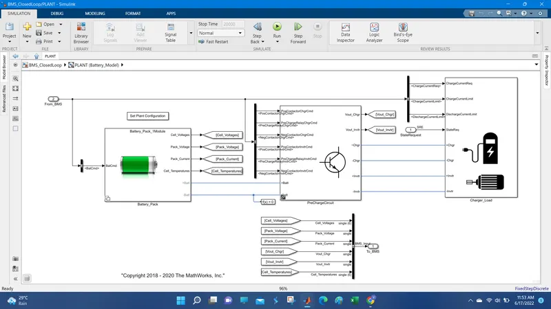
The above figure shows the Plant subsytem. The battery model consists of the Battery pack, Precharging circuit and the charger and load. The battery pack consists of two configuration as 1 module of 6 cells and 16 modules of 96 cells. Here the 1 module 6 cells configuration is chosen since it requires less simulation time. The pre-charge circuit ensures the current to flow in a controlled manner until the voltage level rises before the contactors can close without causing damaging current spikes to the battery.
1)
Case 1:
Select Test case as 1 from the Test sequence variant selector parameters.
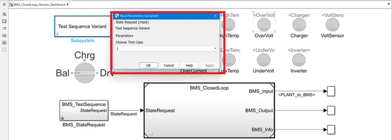
The case selection changes the state request of BMS test sequence.
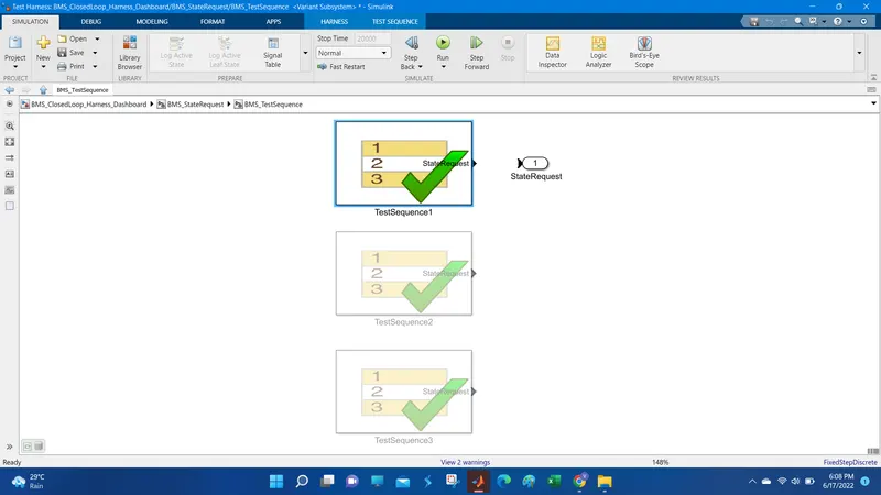
This test case when explored consist of the following sequence of operations.
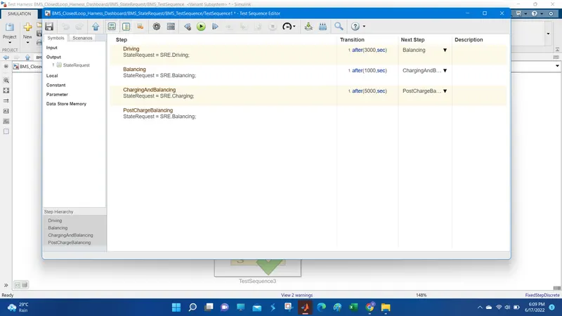
According to this case:
- For the first 3000s the system is driving stage.
- For the next 1000s balancing of cells occurs.
- It is followed by charging and balancing for another 5000s.
- After this for the rest of the simulation period balancing occurs.
Results:
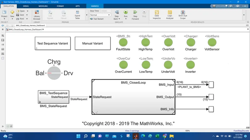
For case 1; all the lamps in the dashboard shows green indicating favourable operation without faults.
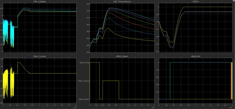
This figure shows the simulation results of test case 1. From Plot 1 of Cell voltages, we can see that for the first 3000s the system is in driving mode hence discharge occurs. The sudden variations or spikes indicate the discharging stage. The cells are at standby position in between 1500 to 2000s in the driving phase. In the driving phase the voltage is reduced from 3.2V to 3.9V. Similar characteristics are observed for the Pack current (plot 2) for the driving phase. For the next 1000s cell balancing occurs and again the cells are at standby phase upto 4000s. Plot 1 and 2 shows similar characteristics during this phase where the pack current goes to zero. After 4000s the cells are now in charging phase followed by balancing phase which shows the current decreasing in Plot 2. The cell voltage attains 4.2V during this phase and the current attains zero at around 7000s. After this for the rest of the period balancing occurs and the pack current maintains at zero and cell voltage settles at around 4.1V.
Now Considering Plot 3 of Cell temperatures During the charging phase the temperature increases from 285 to 295 and remains constant during the stand by period and increases again upto 302 and then remains constant for the balancing phase. Then it again starts to increase at 4000s and attain a maximum of 318 during the charging phase. For the rest of the period as balancing occurs the temperature slow;y decreases.
Considering Plot 4 of BMS state we know that for the first 3000s the system is driving stage. For the next 1000s balancing of cells occurs. It is followed by charging and balancing for another 5000s. After this for the rest of the simulation period balancing occurs.
Considering Plot 5 of SOC, initialy the SOC of battery module is 80%. Here the yellow line indicates the SOC estimation by coulomb counting. Blue represents SOC estimation with unscented Kalman filter (UKF) and Red represents SOC estimation by extended Kalman filter (EKF). Among them UKF and EKF estimation shows promising results. Initialy during the driving phase the SOC decreases to 60% and after the standby stage it further decreases to 45%. During the charging phase it increases to around 85% and remains there during the balancing phase.
Considering Plot 6 of Balancing command, Initially upto 3000s during the driving phase balancing does not occurs. After that till the simulation stops BMS gives balancing command. Balacing occurs for cell 6 (blue) since its voltage is higher than other cell voltages.
Case 2:
Select Test case as 2 from the Test sequence variant selector parameters.
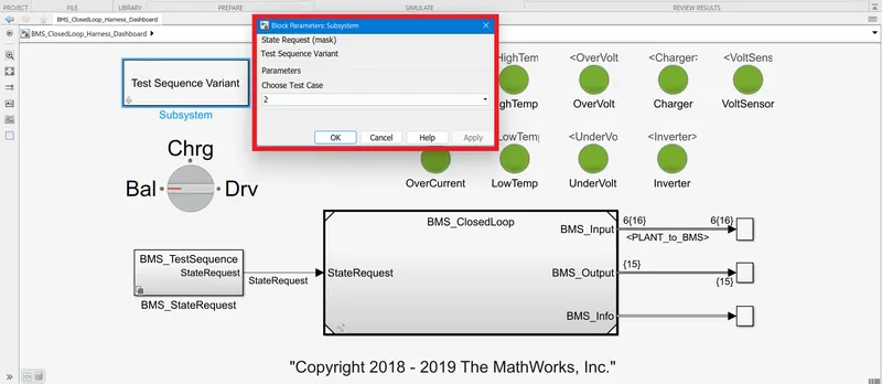
The case selection changes the state request of BMS test sequence.
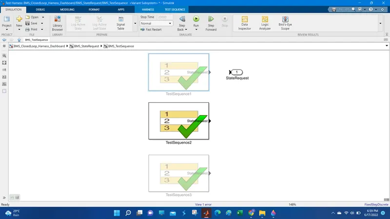
This test case when explored consist of the following sequence of operations.
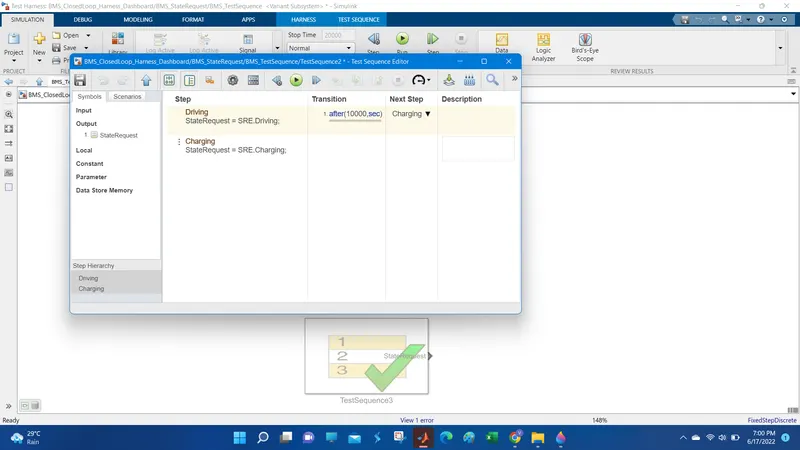
According to this case:
- For the first 10000s the system is in driving phase.
- for rest of the simulation period the cells are in charging phase.
Results:
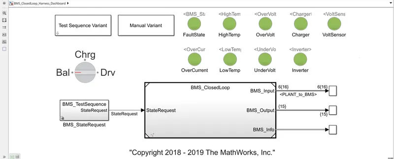
The dashboard results shows no faults as the lamps are all green.
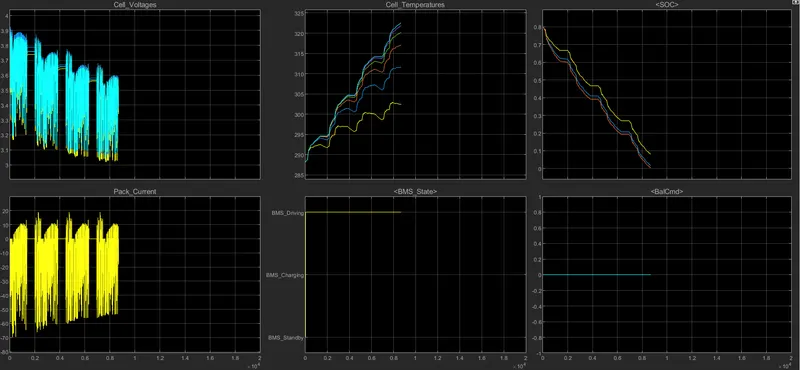
Here we can see that the simulation stops at around 9000s since the battery has completely drained.
From Plot 1 of cell voltages we can see that for the entire 10000s driving phase the cell voltage reduces to around 3V. There are certain standby stages observed in between the driving phase. From Plot 2 of pack current we can follow a similar pattern. From plot 3 of cell temperature cell 6 has attained a maximum temperature of 322 along the driving phase for 9000s. Lowest value attained by cell 1 which is around 300.
From Plot 4 we can see that for the entire 10000s the system is under driving phase. From Plot 5 of SOC we can see that initially the cells are at 80% and decreases steadily and at 9000s the SOC touches 0%. From Plot 6 we can see that balacing command is nil as the system is still under the driving phase.
Case 3:
Select Test case as 3 from the Test sequence variant selector parameters.
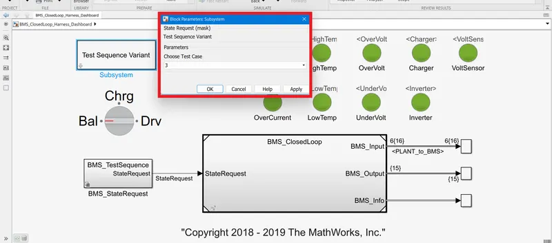
The case selection changes the state request of BMS test sequence.
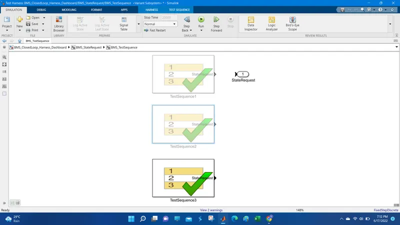
This test case when explored consist of the following sequence of operations.
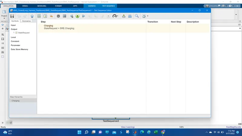
According to this case:
- The entire 20000s of simulation time the system is in charging phase.
Results:
The dashboard results shows no faults as the lamps are all green.
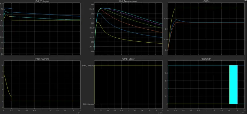
From Plot 1 of cell voltages we can see that for the entire 20000s simulation time charging phase the cell 2 voltage rises to a maximum of 4.2V and then decreases at around 2000s to 4.15V. Other cells also shows the same characteristics but other cells settles at 4.1V after the simulation stop time. From Plot 2 of pack current when the voltage rises the current falls to zero at 2000s and then settles at 0. Indicating current cut-off at full charge condition.
From Plot 3 of cell temperature cell 6 attains a maximum of 292.5 and then decreases to 290 after 20000s of simulation stop time. Similar pattern but decreases temperatures are observed for other cells. From Plot 4 we can see that for the entire 20000s the system is under Charging phase. From Plot 5 of SOC we can see that initially the cells are at 80% initially and increases to around 93% for EKF and UKF SOC estimation responses and for coulumb counting the cell attains 100%. From plot 6, the balancing command for cell 6 can be seen till 18000s after reaching 4.1V the balancing command for cell 2 is observed.
2)
Couomb Counting:
The Coulomb counting approach is linked to continuous monitoring of the input and output currents. Because capacity is the integral of current with respect to time, the change in capacity or capacity deterioration of a battery can be simply determined by measuring the input and output current. SoH is calculated using this method by dividing the measured capacity (after the battery has been discharged to 0 percent SoC value) by the rated capacity. Because of its simplicity, it is widely utilised by scholars. However, this method's accuracy isn't very good. As a result, a clever coulomb counting approach has been created to precisely estimate both SoC and SoH. The most common method for computing the SOC is the coulomb counting method, also known as ampere hour counting and current integration. To calculate SOC values, this method uses battery current readings that have been mathematically integrated across the usage period.

where SOC(t0) represents the starting state of charge, Crated represents the rated capacity, Ib represents the battery current, and Iloss represents the current used by the loss processes. The remaining capacity is then calculated using the coulomb counting method, which simply adds up the charge moved in and out of the battery.
The precision of this method is based on exact battery current monitoring and correct estimate of the initial SOC. The SOC of a battery can be measured by integrating the charging and discharging currents during the working periods with a predetermined capacity, which may be remembered or first estimated by the operating conditions. In the charging and discharging cycle, however, the releasable charge is always smaller than the stored charge. In other words, during charging and draining, there are losses. These losses, together with the self-discharge, result in an accumulation of mistakes. These aspects should be considered for a more accurate SOC estimation. Furthermore, the SOC should be recalibrated on a regular basis, and the declination of the releasable capacity should be taken into account for a more precise calculation.
From the BMS ECU subsystem we can see the SOC estimation block in which the SOC is estimated in 3 methods: Coulomb counting, UKF and EKF using kalman filters.
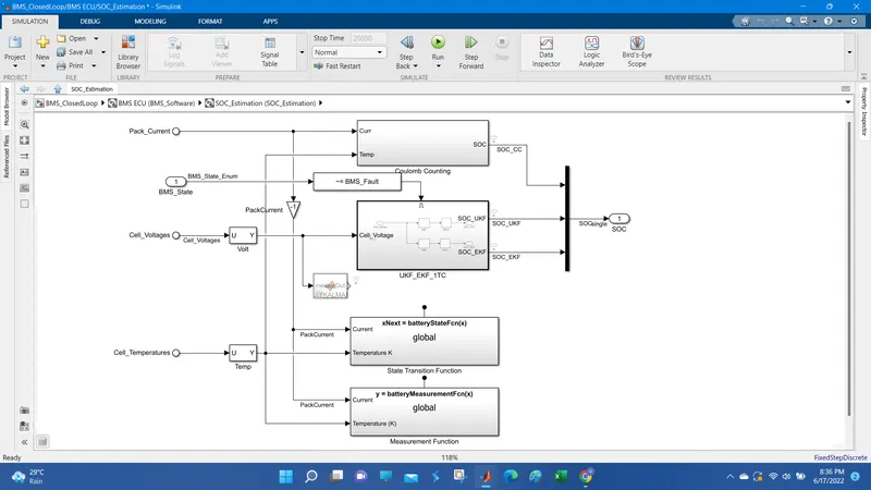
we can see that the only inputs to the Coulomb counting block is the Pack current and Cell temperature. When exploring the block gives:
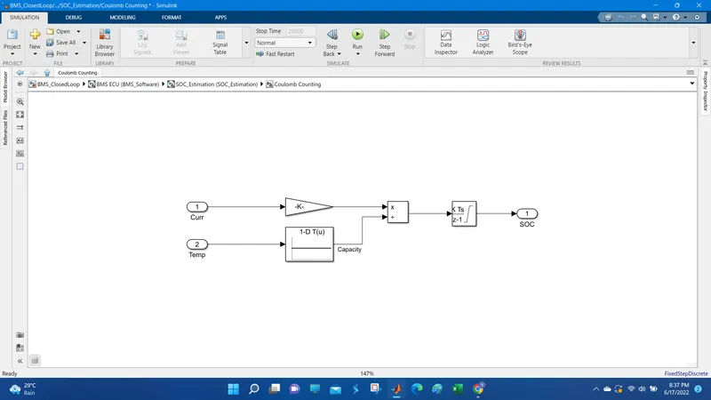
From the equation of coulomb counting method we can see that it is related to the previous SOC and capacity and current. Here we can see that capacity from the lookup table is divided with the current which is multiplied with a gain value. And integrating this value with a discrete time integrator gives the SOC of the battery pack.