Week-11 Challenge: Braking
1)
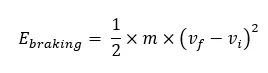
Braking requires some energy similar to that of energy required for accelerating the vehicle. The Braking energy can be calculated by:
 (1)
(1)
Where, Eb is the energy used for braking (J), Vf is the final velocity in m/s, Vi is the initial velocity in m/s and m is the mass of the vehicle.
For a defined driving cycle given below the braking energy is found out using excel calculator;
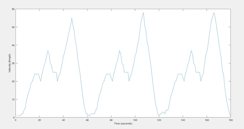
From this driving cycle, we have to first find the braking intervals or intervals when deceleration occurs.
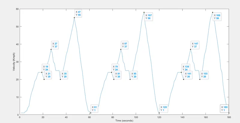
From these data points, the initial and final velocities of different braking intervals can be found out and can be used to find the braking energy using the above equation.
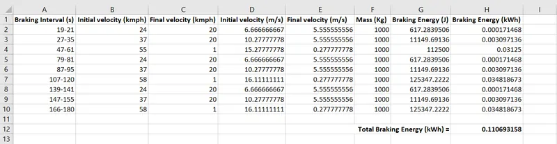
First we need to convert the velocities into m/s, this is done by multiplying kmph value with 5/18. After finding out the the braking energy in Joules using equation (1), we need to convert it into kWh by dividing the energy in Joules by 3600000. After finding out the braking energy of the defined driving cycle for each braking interval, the total braking energy in kWh is found out by taking the sum of all the braking energy in kWh of each intervals.
The total braking energy of the vehicle for the specific driving cycle is obtained as 0.11069 kWh.
2)
Regenerative braking is similar to the transfer of kinetic energy into potential energy to slow down the vehicle,and also charging the battery of the vehicle. Multiple methods are available for this energy conversion and commonly used devices are flywheels. They are installed along the drive train and reduce the motion of the wheels using magnetic fields or mechanical torque. This method differ from mechanical braking cause the energy is used for a cause unlike it is wasted in mechanical braking. Regenerative braking improves fuel consumption and efficiency of the vehicle.
Regenerative braking allows electric vehicle to use the motor as generator when acceleration is not applied and to transfer the energy to a storage system. Driving range of an EV can be extended with the usage of regenerative braking. The regenerative braking torque cannot provide all the required braking torque as it may causes instability of the vehicle. The acceleration torque will always be much higher than the braking torque.
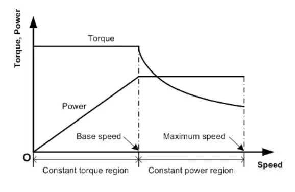
From the torque-speed curve, during low speeds the torque is high and constant. After reaching the critical point the torque gradually decreases and this region is known as the constant power region. Hence at higher speeds the motor is in the constant power region and the values of torque are limited to a low value. Hence it limits the amount of braking torque used for regeneration. But while starting the motor, speed is less and motor will be operating in constant torque region hence high torque is observed. Therefore, braking torque at high speed is less than the at starting of an electric motor.
Co-ordination of Electric and Mechanical brakes:
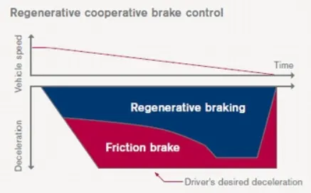
The regenerative braking has limitation under high SOC or at high temperature and hence mechanical brakes need to be implemented to cover the braking torque. Therfore combination of both are used on certain cases, There are two different combination control startegies for braking:
Series Control Strategy: This control stategy is the combination of friction based mechanical braking system with regenerative braking system that transfers the energy to the battery. Here the braking torque is provided or distributed between the regerative and mechanical braking system. Series strategy have good torque blending capability and increases fuel efficiency by 15-30%.
Parallel Control Strategy: Here both the braking systems are used simultaneously without an integrated control. The regenerative braking force is added to the mechanical braking force which cannot be controlled.
Example for braking combination:
EDIB (Electric Driven Intelligent Brake) in Nissan leaf allows the control optimization of regenerative and mechanical brakes. The system focuses on producing an adequate braking force keeping energy generation increased as much as possible. Here at higher speeds, a combination of bith braking systems are used and at lower speeds, regerative braking is given priority.
3)
In motors while considering efficiency we first need to consider the losses. The output mechanica power is given by the input power - the losses. The losses are mainly classified into four:
1.Copper losses: (I²R) represents the overall copper losses incurring in the motor. Here R represents the armature resistance and I is the current. Torque is proportional to current and hence copper losses can be considered as :
Copper losses = Kc x T²
2.Iron losses: Iron losses occurs due to the magnetic losses and can be denoted as:
Iron losses = Ki x ω where, Ki is based on magnetic field effect.
3.Windage losses: Based on the size and shape of the motor, the windage losses are considered.
Windage losses = Kw x ω³
4.Constant losses: These losses are present in the motor constantly and is denoted by C.
Total losses can be found by:
Total losses = Kc x T² + Ki x ω +Kw x ω³+C
Input power = Output power + Total losses
Efficiency = Output power/Input power
The below code plots the contour of given motor speed, torque and efficiency values.
clear all
close all
clc
%Contour plot
x=linspace(1,1000); %speed in rad/s
y=linspace(1,250); %torque in Nm

%Motor loss Constants
Kc=0.2; %Copper loss constant
Ki=0.008; %iron loss constant
Kw=0.00001; %winding loss constant
C=20; %Constant motor losses

[X,Y] = meshgrid(x,y);
Pout=(X.*Y); %output power
Cu=(Y.^2)*Kc; %copper losses
ir=(X*Ki); %iron losses
wi=(X.^3)*Kw; %winding losses

Pin = Pout+Cu+ir+wi+C; %input power
Z = Pout./Pin; %efficiency
V = [0.70,0.80,0.85,0.90,0.91,0.92,0.925,0.93];
box off
grid off
[c,h]=contour(X,Y,Z,V);
xlabel('Speed(rad/s)');
ylabel('Torque(N/m)');
clabel(c,h);
Explanation:
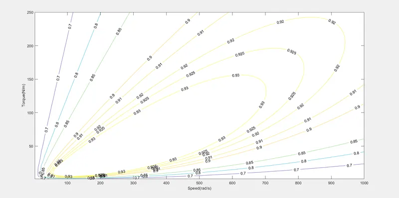
Contour plot shows a 3-D surface in 2-D plane. From the graph we can observe torque in y axis and speed in x axis. The output plots various efficiency values determined in the question for the respective torque and speed values. The contpur plot represents the operational condition of the PMDC motor. The efficiency is higher at lower values of speed and torque and the efficiency decreases as speed and torque values increases.