Week-4 Challenge WOT Condition Part-2

1)

Powertrain blockset in MATLAB/Simulink basically provides two types of models, Mapped and Dynamic Model. Mapped model also known as Static model represents macro level behaviour based on a set of lookup tables. Dynamic model represents actual components or actual data of the engine, motor or generator.

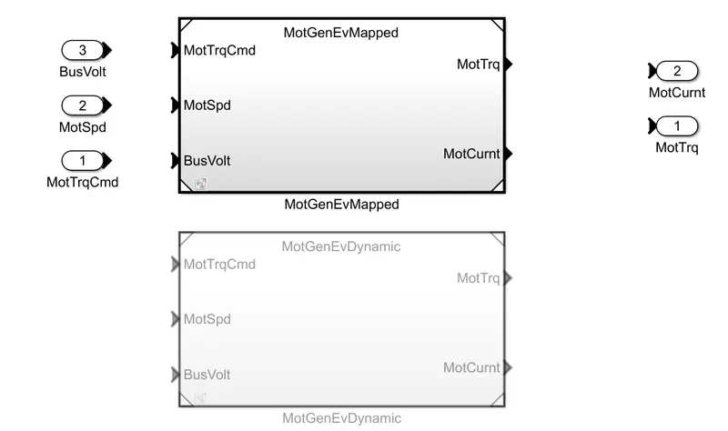
Mapped Model: Here the performance parameters are measured based on 2-D lookup tables. The table shows overall engine characteristics which includes actual torque and fuel flow rate.This lookup data are mainly output of certain experiments that can be used to verify certain conditions and is not apt for real-time conditions. Mapping models gives fast simulation results when compared to Dynamic model. 

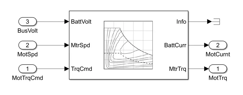
Here, the Mapped Motor block implements a mapped motor and drive electronics operating in torque-control mode. The output torque tracks the torque reference demand and includes a motor-response and drive-response time constant. Use the block for fast system-level simulations when you do not know detailed motor parameters, for example, for motor power and torque tradeoff studies. The block assumes that the speed fluctuations due to mechanical load do not affect the motor torque tracking. This is an example for Mapped model in Electrical Vehicle.

Dynamic Model: It represents the actual components of the motor/generator and engine and understands the behaviour my decomposing to multiple components inorder to describe and predict the interactions of the system over time. Suitable for real-time analysis. Simulation results takes time when actual components are involved. An example for dynamic model of a motor is shown in case of Electric vehicle.

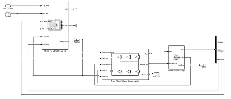
Here, the actual components i.e, the 3-phase motor and inverter units are included rather than pre-defined experimental data or lookup tables. We can change any parameters to get real-time analysis of the system with dynamic models involved.

To switch between Mapped and Dynamic model with reference to EV model:

a) Open the EV reference model by using the command 'autoblkEvStart'.

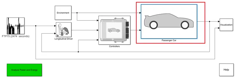
b) Select the 'Passenger Car' block.

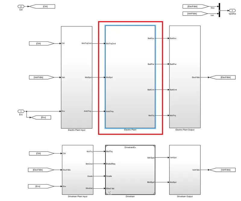
c) Now select the 'Electric Plant' Block.

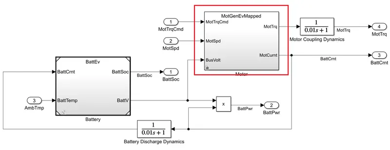
d) Now right click on the 'Motor' Block and select the 'varient' option as shown below.

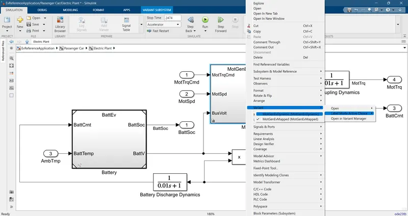
Now by selecting 'MotGenEvDynamic' the model gets changed to dynamic model from mapped model.

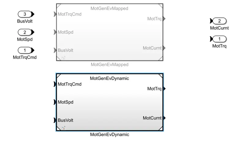
Hence we can change between Mapped and Dynamic model by using the following steps in EV reference model.

2)

MPGe stands for Miles Per Gallon Equivalent is a unit formulated by the US inorder to compare the fuel efficiencies of Battery cell EVs, Plug-in hybrid EVs and Fuel cell EVs. For conventional gasoline vehicle, the fuel effciency is calculated by Miles Per Gallon (MPG). MPG is the number of miles you can drive per gallon of gas. In terms of energy,1 gallon of gas is equivalent to 33.7 kwh of Electricity. This is useful when the engine can use an alternative source of fuel which cannot be measured in terms of liquid gallons of fuel. 

Eg. If a battery powers the vehicle for 4 miles/kwh capacity of battery. so, in terms of miles per gallon:

4 miles/kwh*33.7 kwh/gallon=134 MPGe.

With reference to the HEV model, In 'visualization' block we can see the MPGe being calculated.

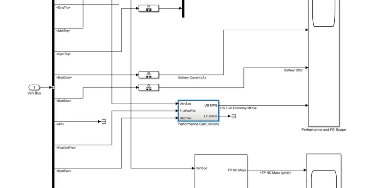
In performance calculation we can see that with the inputs vehicle speed,Fuel volume flow and battery power, the MPGe value is calculated. In case of EV there will only be vehicle speed and battery power as inputs to find out MPGe.

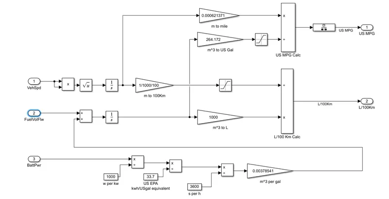
Steps to find MPGe includes:

• The battery power is first converted from watts to kWh by dividing the power in watts by 1000
• Then to find the gallon equivalent we need to divide the battery power in kWh by 33.7 to get in kWh/gal.
• To convert kWh/gal in terms of seconds that is kWs/USgal divide the gallon equivalent by 3600.
• Now convert kWs/gal to  mᶟ/gal by multiplying it with 0.00378541.
• Now we add the Battery power with Fuel volume flow and integrate it with respect to time.
• Then multiply the output with 264.172 to convert it from mᶟ to US gallons let this be (1).
• Now to find the distance covered by the vehicle in miles, Square the vehicle speed inorder to remove all the negative values due to deceleration and then find the root to get the vehicle speed.
• Now by integrating the vehicle speed with time we get the distance covered by the vehicle.
• Then convert the distance in m to distance in terms of 100 km. i.e, D/1000/100
• Then the final step is to convert the distance into miles by dividing the distance in 100 km with 0.000621371. A saturation block is provided to get values greater than a certain limit. Let this be (2).

From these two values the MPGe value is foud out by dividing (1) by (2).

Factors affecting fuel flow:

In Mapped model the fuel mass flow (kg/s) is given as input to the engine in the form of lookup tables. Whereas in case of Dynamic model or actual model the fuel flow depends on the factors such as Stoichometric air-fuel ratio, Specific gravity of fuel and Lower heating value of fuel.

3)

To run the HEV reference application with WOT drive cycle. First open the HEV reference application using 'autoblkHevStart' Command.

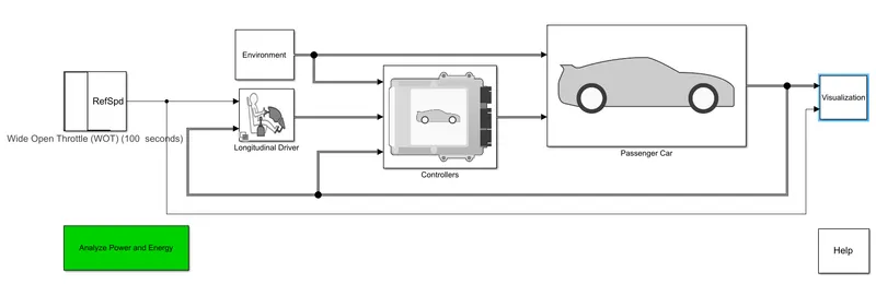
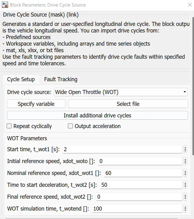
 Now set the drive cycle to WOT condition and vary the drive cycle parameters according to our needs.

Now select the 'Environment' block and change the grade and wind speed to 10 and 6 respectively.

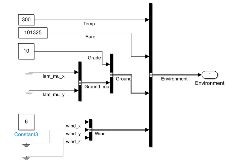
Now run the simulation and get the results.

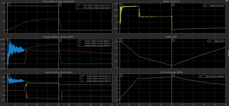
From the plot we get the following results:

Trace velocity target and Actual Plot: The yellow line indicates the desired input or the step input given. The blue line, the actual vehicle speed should trace the input or should attain the max speed with reference to the input at a certain instant of time. But vehicle doesn't attain the max speed because the energy sources weren't able to provide the required power to the vehicle due to their limits due to the presence of grade and wind speed. Hence the Max speed attained by the vehicle is 63 mph at a duration of 45 seconds.

Battery current Plot: When the vehicle is accelereating the battery current also increases and reaches the max discharge limit possible. When the battery SOC reaches below 70% there is a sudden decrease in battery current and remains constant at a new limit while the Engine powers the vehicle. After 50 sec, during deceleration the battery current goes to negative indicating charging of battery. The discharging limit of the battery is usually greater than the charging limit. Here the discharging limit is around 510 A and charging limit is around -260 A.

Battery SOC Plot: Here the battery SOC depletes until deceleration happens and due to regenerative braking the battery SOC increases. The battery SOC toggles between 60% and 80% here. The SOC at the lowest point is 61% before increasing.

Engine, Motor and Generator Speed Plot: Due to the high initial torque provided by the motor it is used to start the vehicle (blue) and when the battery SOC falls below 70% Engine kicks in powering the vehicle and generator(red) charges the battery during deceleration. Engine and Generator speeds are overlapped and hence seen as red in the plot. Max speed of motor is given by 7781 rpm and Max speed of engine is given by 5360 rpm.

Engine, Motor and Generator Torque Plot: Motor torque (blue) is high at first and then engine torque(yellow) kicks in when the battery SOC reaches below 70%. Motor torque is negative at deceleration part indicating charging of battery. Generator torque (red) indicates charging the battery.

US Fuel Economy MPGe Plot: Maximum fuel economy achieved is 5.723. And a decrease is noticed in fuel economy when the battery SOC decreases from 70% to 65%.

4)

First open the EV reference application by using 'autoblkEvStart' command and chnage the parameters similar to the HEV parameter updation for the WOT and Environment Block by keeping all other parameters constant.

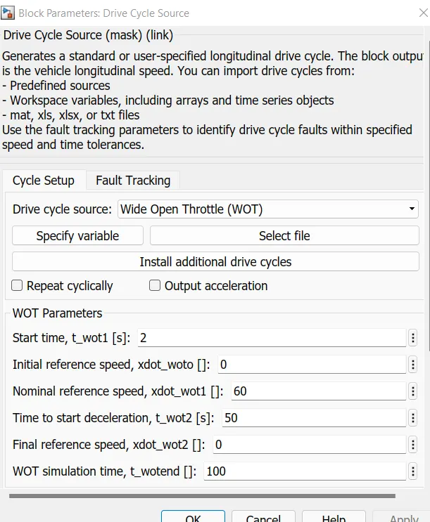
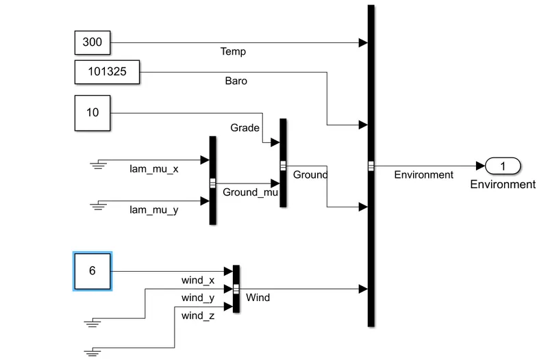
Now run the simulation and get the results and compare it with HEV performance.

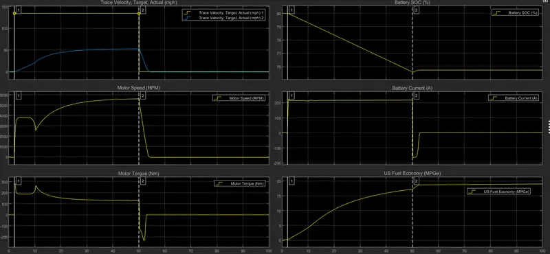
By Comparing the plots of HEV and EV:

1. The first plot is almost the same since motor was operating during the initial region in HEV due to high initial torque. Here also the vehicle is unable to achieve the max speed with respect to the input because of the discharging limit of the Battery. Here the max speed attained by the vehicle is 53 mph at a duration of around 45 seconds.
2. The battery current drawn or the discharging limit of the battery in HEV was around 510 A and reduces further as the load is met by engine or when the engine kicks in. In case of EV it is around 217 A. It can be noted that the negative current or regenerative braking happens in HEV for a longer period compared to EV. The charging limit is around -162 A in EV.
3. SOC increases in HEV at 15-20% during deceleration or regenerative braking but in EV the percentage improvement is less than 2%. This can be explained with respect to the period of negative battery current mentioned above. Here the SOC at lowest point is around 75%.
4. Motor speed is stable without much fluctuations in EV compared to HEV. Max. Motor speed in HEV was around 7781 rpm whereas in EV it is 5620 rpm. Motor speed decreases for a short period of time during deceleration and goes to zero in EV.
5. Motor torque in EV is much stable compared to HEV which has large fluctuations during starting. Similar to HEV during deceleration the motor torque goes negative in EV indicating charging of battery.
6. Maximum Fuel economy of HEV was around 5.723 whereas in EV this is around 18 which shows that fuel economy of EV is significantly greater compared with HEV. This is because the Electric motor is much more efficient than the Engine.