Week 7 State of charge estimation

https://in.mathworks.com/matlabcentral/fileexchange/72865-design-and-test-lithium-ion-battery-management-algorithms

1.Simulate the 3 test cases from harness dashboard and write a detailed report on the results

2.What is coulomb counting? Refer to the above model and explain how BMS implements coulomb counting for SOC estimation ?

Hint :(Download the file from the link and go to SOC estimation model-ECU block).

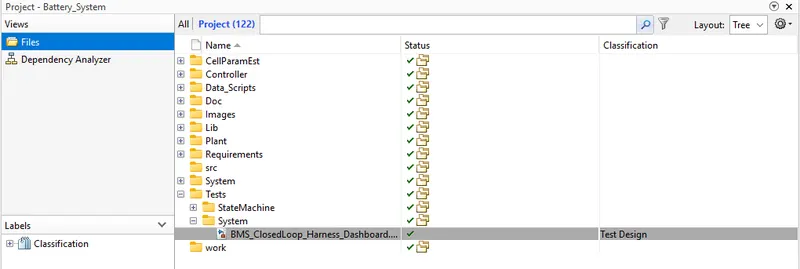
Solution: First click on the link and download the MATLAB file for the simulation of model Under the three test cases from harness dashboard. After downloading the file. Exatract it, then go into the file and again extract the zip file according to the version of MALAB you are using. And then go to MATLAB and open this file, where we can see all the data about the simulink models. From the model under the opened file, click on tests and in that open the BMS_closed loop_harness dashboard, which is shown in the following image. Then simulate the 3 test cases.

Before this i have selected only for pack1 of the battery so that my output will be clear. As mentioned in the folowing way, First open the BMS_system from the project shorcuts which is at the top of window as shown in the following image.

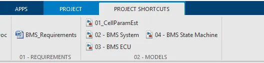
After selecting the BMS_system, click on plant configuration and select the pack 1.

1.Simulate the 3 test cases from harness dashboard and write a detailed report on the results.

By opening the model BMS_closed loop_harness dashboard, will get the following figure .

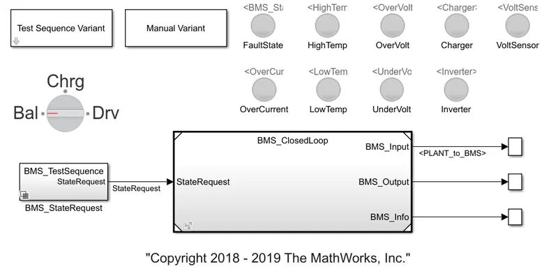
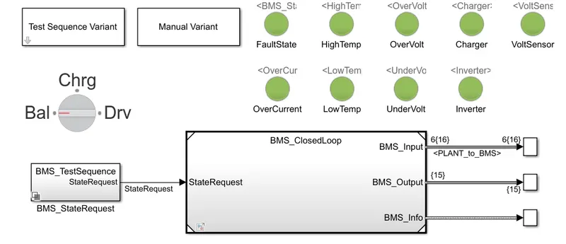
In the above figure observe the different block which perfoem different functions. Which are explained below.

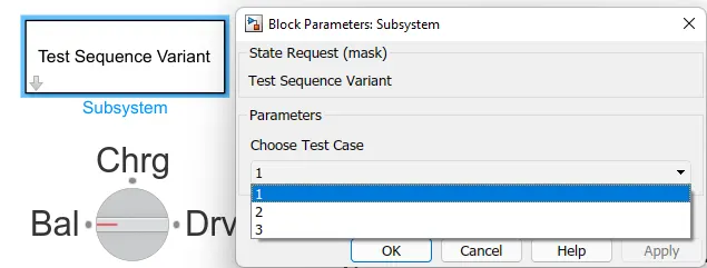
Test Sequence Variant block is used to choose the test case. Manual varient is used to operate manually under certain situations. The following figure shows the test sequence variant block subsystem to choose the tests. In the first case will select 1.

Bal.charge.Drv block represents the conditions of the vechile which is used under this BMS. When is indicates Bal, it means the vehicle is in balancing condition. If it indicates Charge. then it is in charging condition. If it indicates Drv. then it means the vehicle is in driving conditions. These variations we can observe while the model is under simulation. The timing for these three conditions will be set according to the test condition. The three conditions are shown with the following figures.

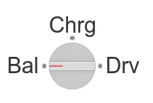
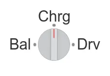
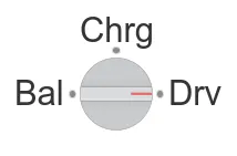
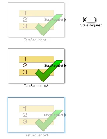
Now coming to the BMS_State request block, it gives which test is to be perfome like if we set the case 1 then the state request will perform the first test and other 2 will be off. Under first test selection, it is shown as below.

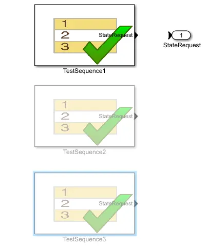
If we click on the test sequence blocks we can see the different timings for the Balance, driving and charging modes. The following figures shows the timing duration set for the test sequence block.

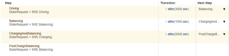
TestSequence1: In this test sequence we can observe that different time trasitions between the modes. Here the drving mode is on for 3000sec and after that balancing condition will activate. After 1000sec charging and balancing condition will accepts. After 5000sec of this conditions post charge balancing mode will activates.

And the lamp block which are attached to the dashboard will indicates the fault happen in any of the aspect. If everything is good then all the lights will be in green colour, if any fault occurs at any condition then the lamp block which represents that condition will glow in red colour. Now will perform the tests.

Test-1: In this case we are selecting the test sequence variant as 1. And simulating the model for 20000seconds. After the simulation, all the lamp block which are taken are glowing in green colour which indicates that there is no fault. So everything will be normal, then we can see all the changes in three modes which are Bal,Drv, and Charg. And also we can observe the SOC variations, temperature of different cells and etc.

After the simulation, the following plot will be observed.

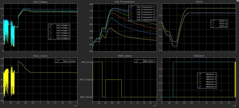
In the above plot we can observe the parameters like Cell voltage, temperatures, SOC, total pack current, BMS state and Bal cmd.

1. In the first plot we can observe that from intial stage to 3000seconds it is in driving mode, so there is voltage fluctuations according the driving conditions. The voltage varies in between the 3.2-3.8V. The nominal voltage of each block is 3.7V. So the maximum variations are happend in between those limits. From 3000-4000seconds the vehicle is in Balancig state, in this mode the voltage of the cells settles at its nominal voltage that is at 3.7V. At the 4000sec the voltage is in increasing mode because after 4000seconds the mode will enters to charging and balancing state for 5000sec means till 9000sec, in this mode the cells gets charged. So it reaches to its full charging voltage i.e, 4.2V and next it enters to postcharge balancing mode where all the voltages get settles to around 4.1V.
2. In the second plot we can observe temperature variations at each cell. So again coming to the modes of operation. That is at driving mode 0-3000sec the temperature of cells starts increasing according to the drive cycle. In balancing condition i.e, 3000-4000sec the temperature of the cells decreases gradually. After that charging and balancing mode will starts from 4000-9000sec, where the temeprature again starts increasing during charging and then starts decreasing for balancing mode. After that there will be only slight decrement in the cell temperatures as it indicates the postcharge balancing mode.
3. This plot shows the SOC changes according to the transition of the modes. In the driving mode the SOC(state of charge) decreases from 80% to 45%. In the balancing mode the SOC gets settled at 45%. After that charging and balancing mode will activates, where the cells gets charged so the SOC will increases to 100% and then settles at full mode in postcharge balancing condition.
4. In this plot we can observe the total pack current, intially in the driving mode we can see the changes in current value according to the drive cycle. It varies from aroud -70A to 10A. When the vehicle eneters into balancing mode then the current of the pack settles at zero. And when charging and balancing mode activates, the pack current will starts increasing it is around 30A and then gradually starts decreasing to 0A. Later on settles at 0A as the vehicle enters into postcharge balancing mode.
5. This plot shows the BMS state. Like in which state the BMS in operating. We can see that on the y axis, three modes are pointed which are Drivig, Charging and Standby. In driving mode i.e, till 3000sec the plot is at driving point. After that for 1000sec i.e till 4000sec, it will be in standby position as it is in balancing mode. Then till 9000sec it represents at charging mode. Then it will settles at standby position which represents the postcharging balancing mode.
6. This plot shows balancing commmands. Lie when the balancing mode activates then plot reaches to 1. So according to the balancing commands the plots will settles.

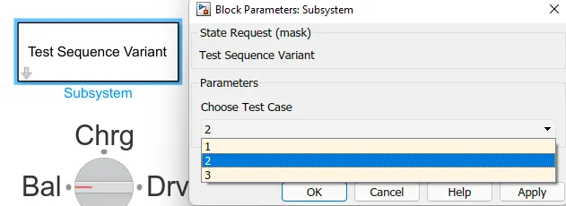
Test-2: Now we have to select the test variant sequence to 2. Which shows in the following image.

After setting this in the BMS_state request second case will activates and remaining two cases will be off. Which is shown in the following figure.

TestSequence2: In this sequence, we can see that only two transitions. Intially driving condition will intiate for 10000sec after this duration charging mode will activates. We can also edit the duration.

After making the changes, simulate the model. After the simulation process, the following figure will represents the model.

The resultant plot has been observed as shown in the following image.

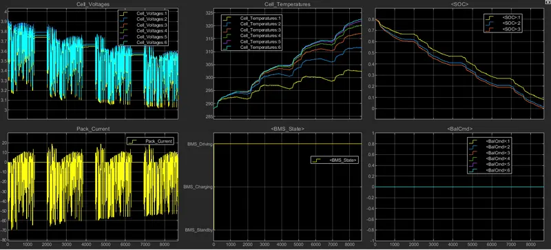
From the above plot, following observations has been identified. Before explaining the plots it should noted that here only 2 modes are happening one is driving mode and then charging mode will activates.

1. From the first plot we can say that is complete driving mode so there is many variations according to the drive cycle. Here the voltage level is varying from 3.2-3.9V intially. But due to the continues driving there is a gradual decrease in the voltage ranges also so we can see that at end the voltage varies between around 3.1-3.7V.
2. In the second plot we can see the temperature of the six cells. As the vehicle is in driving mode, the temperature is continuously increasing due to the high running time.
3. From the SOC plot we can observe that, the SOC is intially at 80%, while driving the SOC is starts discharging, even though there are charge and discharge conditions in the driving mode the running time is high so the SOC is reached to its 0% at 8692seconds. So its not even completed its driving duration also. Which we have set for 10000sec. So all the plot stops at that time because at 0% SOC the vehicle stops then there is no other changes.
4. In the pack current plot, we can see the current variations according to the drive cycle.Intially it is varying between -70A to 15A. But to the long running time the current value also come to around -55A to 20A. And it ends after SOC reaches to 0% as there is no charge to supply.
5. This plot shows the BMS state of operation. As we discussed till now we have only seen the driving mode. So that is why the plot maintains its consistency at Driving mode.
6. In the last plot we can see the Balcmd. Since there is no balancing mode it settles at 0 only.

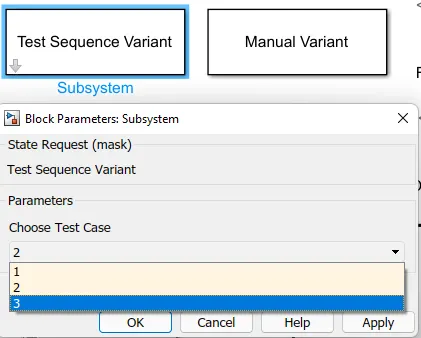
Test-3: Now we have to select the test variant sequence to 3. Which shows in the following image.

After setting this in the BMS_state request third case will activates and remaining two cases will be off. Which is shown in the following figure.

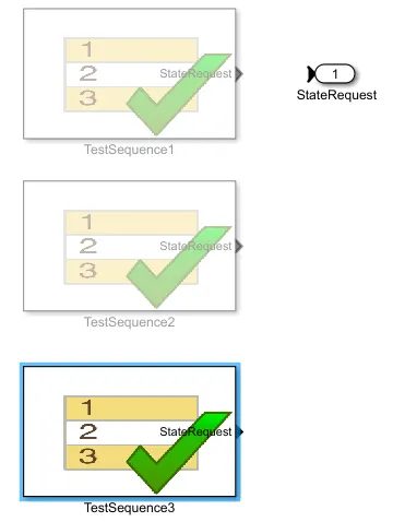
TestSequence3: In this sequence, we have set only charging condition throughout the simulation. So will see the resultant plots according to the siulation.

After making the changes, simulate the model. After the simulation process, the following figure will represents the model.

The resultant plot has been observed as shown in the following image.

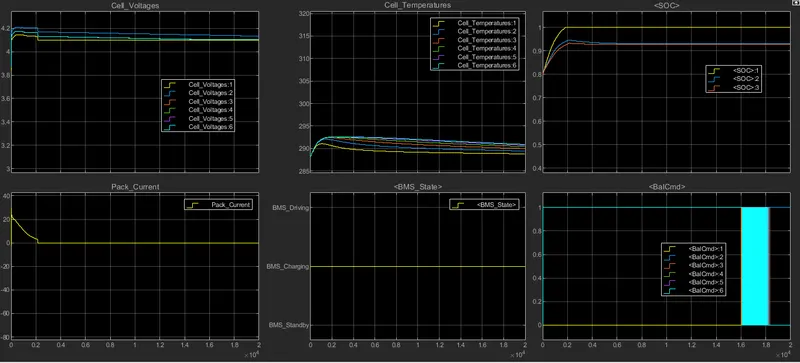
From the above plot, following observations has been identified. Before explaining the plots it should noted that here only 1 mode is happening that is at charging mode. This is as we set in the test sequence3.

1. So from the first plot we can see that, it reaches to full load voltage that is 4.2V and then a small decrease to 4.1V and maintained that value through out the simulation. As this is only charging mode there is no change in the voltage of the cell.
2. From the temperature plot, it can be observed that while battery is in charging condition there is a increment in the temeperature of the cells. But after the battery is full charged the temperature values are quitely settled at normal temperature.
3. In SOC plot we can observe that, it is charged from 80% to 100% in 2000seconds and then it maintains its constant 100% throughout the simulation.
4. From the pack current plot it can be say that, while battery is in charging mode there is a rise in current from 0A to 20A, but after the battery gets fully charged the pack current comes to 0A and then settled.
5. The mode in this case is only charging so the BMS state plot shows only the charging mode.
6. As there is only charging mode, the balancing mode maintains at 1. Which shows in the last plot.

2.What is coulomb counting? Refer to the above model and explain how BMS implements coulomb counting for SOC estimation ?

Coulomb counting: The Coulomb counting method measures the discharging current of a battery and integrates the discharging current over time in order to estimate SOC. Coulomb counting method is done to estimate the SOC with respect to time. Which is estimated from the discharging current I(t), and previously estimated SOC values, SOC(t-1). SOC is calculated by the following equation.

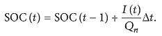
But there are several factors that affect the accuracy of Coulomb counting method icluding temperature, battery histort, discharge current and life cycle. Coulomb counting method depends on the recording of the current noise only. The signal is filtered with a high pass filter with a cut off frequency of 0.01Hz. The filter may b either analogue or digital. The absolute value of the measured current samples is then summed over time. A steep slope is taken as an indication of rapid corrosion, although it is not possible to calibrate this in terms of an estimated corrosion rate.

Modified Coulomb Counting method: To improve the Coulomb counting method, a new technique called modified Coulomb counting method is proposed. The modified Coulomb counting method uses the corrected current to improve the accuracy of estimation. The corrected current is the function of discharging current. There is a quadratic relationship between the corrected current and discharging current of battery. By practice of experimental data, corrected current is calculated by the following formula,

where k1, k2 and k0 are constant values which are obtained from the practice experimental data. In modified Coulomb counting method, This method employs battery current readings mathematically integrated over the usage period to calculate SOC by the following equation,

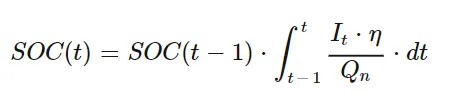
where,

SOC(t-1) = SOC at previous time step,

η = Efficiency,

t = Current time step,

Q = Charge capacity of the battery.

The experimental results shows that the accuracy of the modified Coulomb countig method is superior to the conventional Coulomb counting method. The Coulomb counting method then calculates the remaining capacity simply by accuulating the charge transferred in or out of the battery.

How BMS implements coulomb counting for SOC estimation in the above model:

BMS implements coulomb couting for SOC estimation in the above, which we can observe in the BMS ECU block. This can be opened by clicking on the BMS_system. The following model will appears if we click on the model.

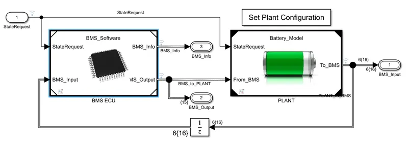
In the above block we can see the subsystem of BMS ECU whic takes the state request and perform the respective operations then gives the information to the Plant of the battery pack. So if we click on the BMS ECU block we can see the following subsystems.

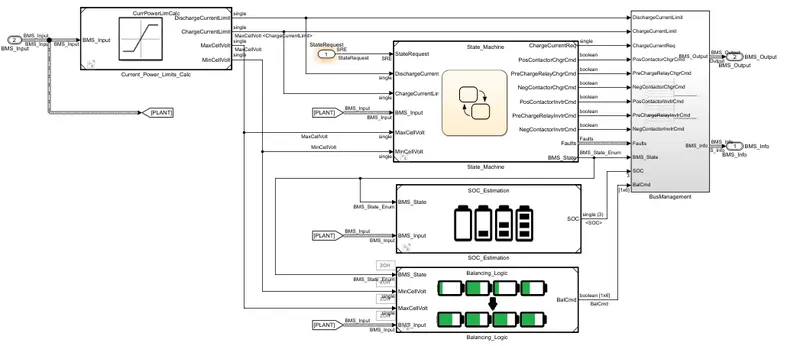
There we can see the current power limits subsytem, state machine, SOC estimation, Balancing logic and BMS controller. Here after performing the respective operation the total information will be given to the BMS management where it will further process the data. In the SOC estimation subsystem will perform all the required formulas or methods to calculate the SOC of the vehicle. And will give this to BMS management from there it will gives us the indication. If we open the SOC estimation then folowing modelling will appears.

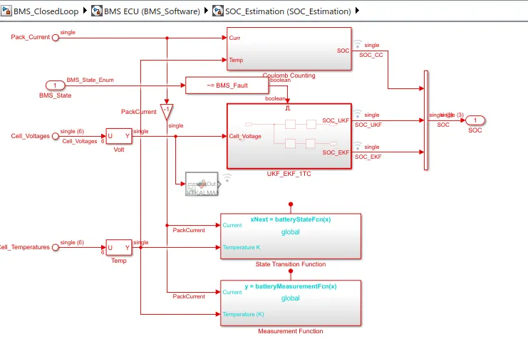
In this subsystem we can see that various methods to estimate the SOC. In this the first block represents the coulomb counting method. Where by using the method will estimate the SOC. If we open that subsystem we can observe what is happpening or what blocks we have taken to estimate SOC and all. The following figure shows the system under Coulomb counting method.

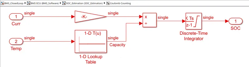
So here we are taking the current and temperature parameters of the cells and giving to the gain block and 1-D lookup table respectively. Where the lookup table gives the capacity over the time. The capacity will vary with respect to the temperature so that is why we have taken the temperature as input to the look up table. Now these outputs from the gain block and look up table is given to the product block, where the gain is multiplied means the current with respect to gain is multiplied. And the capacity has been integrated. That output is given to the discrete time integrator block, it performs the integration operation and gives the value of SOC. As we discussed before it applying the formula here over the current and capacity.

The Coulomb counting method is associated with monitoring the input and the output current continuosly. Since capacity is the integral of current with respect to time, by measuring the input and the output current, change in capacity or capacity degradation of a battery can be measured easily. In this metho, we calculated by dividing measured capacity(after discharging the battery to 0% SOC value) to its rated capacity. It is an extensively used method by researchers for its simplicity. But, the accuracy of this method is not very high. The main advantage of Coulomb counting is its simplicity, easy implimentation and low computational cost.