Project

Aim: To study, analyze and prepare a technical report explaining the model properties of Baja ATV model.

First we are going to know What is ATVs:

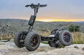
An All-Terrain Vechile(ATV) is defined as a motorized off highway vechile designed to travel on four low pressure or non-pneumatic tires, having a seat designed to be straddled by the operator and hadlebars for steering control. It is designed to handle a wider variety of terrain than most other vechiles. The rider sits on and operates these vechiles like a motorcycle, but the extra wheels give more stability at slower speeds. Although most are equipped with 3 or 4 wheels, 6 wheel models exists and existed historically fo specialized application. Multiple user analogues with side by side seating are called Utility Terrain Vechile(UTV) to distinguish the classes of vechile. ATVs are used in agriculture to bridge the advantages of trucks and tractors. They are used in a variety of industries for their maneuverability and off-roading ability. They are also used in land management. military, emergency medical services and etc,. Sport modes are built with performance, rather than utility. To be successful at fast trail riding, an ATV must have light weight, high power, good suspension and a low center of gravity. These machines can be modified for such racing disciplines as motocross, wood racing, desert racing, hill climbing. ice racing and others. The following image shows the model of ATV.

BAJA SAE:

Baja SAE is an intercollegiate engineering design competiotion for undergraduate and graduate students. The main objective is to simulate real world programming design projects and their related challenges. The students must function as a team to design, build,test, promote and compete a vechile within the limits of the rules. Each teams goal is to design and build a prototype of a rugged, single seat, off road recreational vechile. The vechile must be safe, easily transported, easily maintained and fun to drive. It should be able to negotiate rough terrain without damage. This Baja SAE competition event consists of 3 to 4 days. The goal in Baja SAE racing is to design, build and race off-road vechiles that can withstand the harshest elements of rough terrain.

Blocks that are used during the simulation process are:

• Signal Builder: To input the brake, throttle and CVT ratio.
• Simulink to PS Converter: To convert the simulink sigal to simscape environment.
• Solver Configuration: To specify the solver parameters before starting the simuation process
• Mechanical Reference: To make sure all the components are clamped to the ground.
• Generic Engine: To run the engine with speed and torque values as input.
• PS to Simulink COnverter: To convert simscape signal to simulink environment.
• Display: To view the calculated engine power.
• Scope: To view the plot of parameters for better understanding.
• Inertia: To represent the solid inertia.
• Variable gear ratio: To vary the speed according to the gear ratio.
• Rotational Motion Sensor: To sense the rotational motion from the engine and give output as RPM.
• PS terminator: Terminator for unconnected physical signal outputs.
• Double Shoe Brake: To apply brake to the vechile when needed.
• PS Constant: To generate constant physical signal.
• Tire: For transportation of the vechile.
• Rotational Free End: For mechanical components(tire).
• Vechile Body: To represent the Baja ATV model.
• Custom measure guage: To measure the brake and throttle input.
• Knob: To increase or decrease of throttle and brake inputs.
• Lookup table: To insert the CVT values from the workspace.
• Simple Gear: To reduce the speed of the engine with pre-defined gear ratio.
• Step block: To increase or decrease an input value for a defined time interval.

Model 1 of BAJA ATV:

Generic Engine: The Generic Engine block represents a general internal combution engine. This block is suitable for spart-ignition and diesel. Speed-power and speed-torque paramterizations are provided through it. A throttle physical signal input specifies the normalized engine torque.

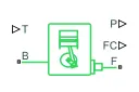
Ports:

• B- Rotational conserving Port representing the engine block
• F- Rotational conserving Port representing the engine Crankshaft
• T- Physical signal input port specifying the normalized engine throttle level
• P- Physical signal output reporting the instantaneous engine power
• FC- Physical signal input port reporting the fuel consumption rate.

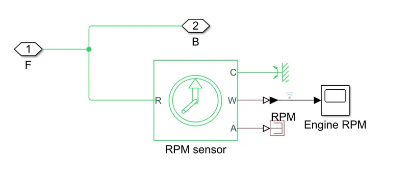
Engine Sensor: The internal block of the Engine sensor is shown in the following image. Where physical signal ports W and A represents the angular velocity and angular displacement of port R relative to port C. The measurement is positive when the motion at R is greater than the motion at C. Where the W port is connected to Scope block through PS to Simulink converter. The Scope measures the Engine speed in RPM.

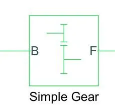
Simple Gear: The simple gear is a combination of Driver and driven gear. If one of these gears is attached to a motor or crank then it is called driver gear. The gear that is turned by the driver gear is called the driven gear. The folowing image shows the simple gear block, where B represents Base gear and F represents Follower gear.

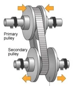
CVT(Continuously Variable Transmission): A continuously variable transmission is an automatic transmission that can change seamlessly through a continuous range of gear ratios. This contrasts with other transmissions that provide a limited number of gear ratios in fixed steps. The fiexibility of a CVT with suitable control may allow the engine to operate at a constant RPM while the vehicle moves at varying speeds. CVTs are used in automobiles, tractors, motorscooters, snowmobiles, bicycles and earthmoving equipment. In CVTs, the variable diameter pulley plays a important role in transmission. Variable diameter pulleys must always come in pairs one of the pulleys known as drive pulley which is connected to the crankshaft of the engine. The driving pulley is also called as primary or input pulley because it's where the energy from the engine enters the transmission. the second pulley is called the driven pulley because the first pulley is turning it as an output pulley. The driven pulley transfers energy to the driveshaft. The variator which is connected to the primary pulley when it goes outward, the variator of secondary pulley will goes inward, then radius of primary pulley is less than radis of secondary pulley which leads to speed reduction and vice versa. In other words, torque ratios are achieved when the belt rotates at the lower cross section of the input pulleys and at the greater cross section of the output pulleys. And speed ratios are achieved when belt roates at the higher cross section of the input pulley and lower cross section of the output pulley. The following daigram shows the Basic structure of the CVT.

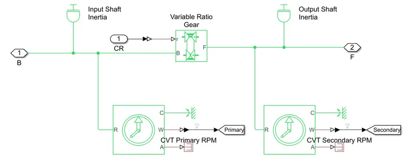
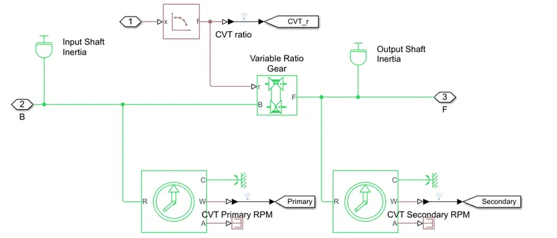
The following image represents the block daigram of the CVT. Where the input shaft inertia and output shaft inertia represents the primary and secondary pulley respectievely. And CVT primary and secondary RPM are the engine sensors. To specify the Gear ratio we have given a variable gear ratio block.

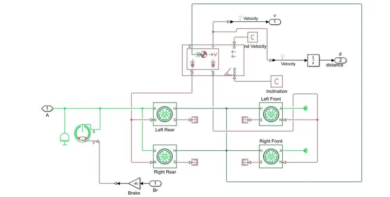
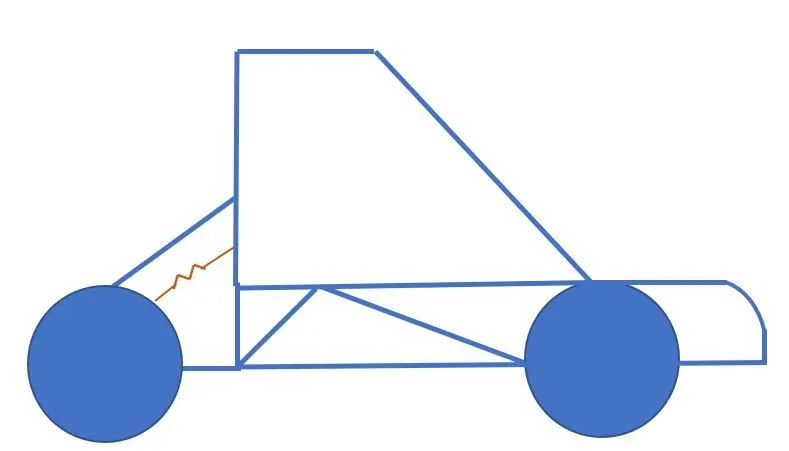
Vechile Body: The Vechile body block represents a two axle vechile body in longitudinal motion. The vechile can have same or different number of wheels on each exle. For example, 2 wheels on the front axle and one wheel on the rear axle. The vechile wheels are assumed identical in size. The block accounts for body mass, aerodynamic drag, road incline and weight distribution between axles due to accelaration and road profile. The vechile does not move vertically relative to the ground. The block has an option to include an externally defined mass and inertia. The mass, inertia and center of gravity of the vechile body can vary over the course of simulation in response to system changes. The following daigrams shows the inner blocks of the Vechile body and basic appearence of it.

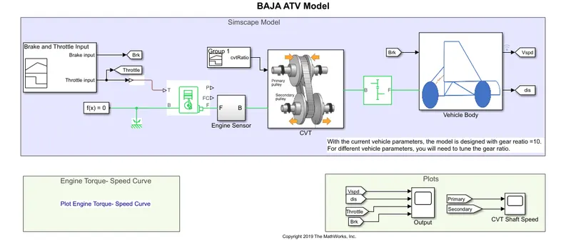
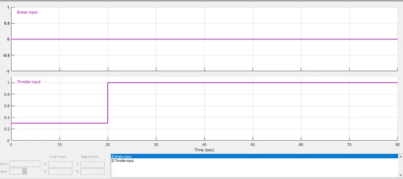
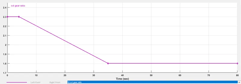
First we have to set the throttle signal through signal builder and input it to generic engine block. The random CVT ratio is set through the another signal builder block to get the value of velocity and give it as input to the CVT block as shown in the following figures.

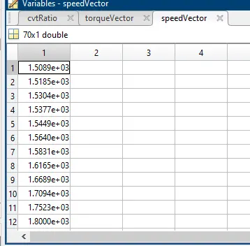
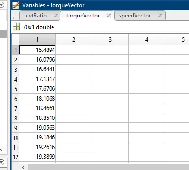
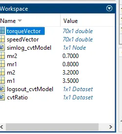
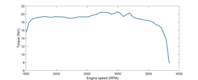
The Torque vector and speed vector values are inputted through the MATLAB workspace which are shown in the following figure.

The engine will generate the output rpm which can be taken from the crankshaft output. This speed will be given to the ideal rotational motion sensor to sense the output RPM. The same output speed will be given to a simple mechanism to reduce the speed where the gear ratio is 4. Then the output speedd from the gear reducer will be given to the CVT. The speed is controlled by the variable CVT ratios. And the controlled output speed is inputted to the vechile axle. The Power from the CVT is inputted to the axle and the vechile accelerates according to the speed. Then velocity is taken as output from the vechile body.

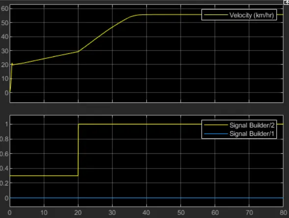
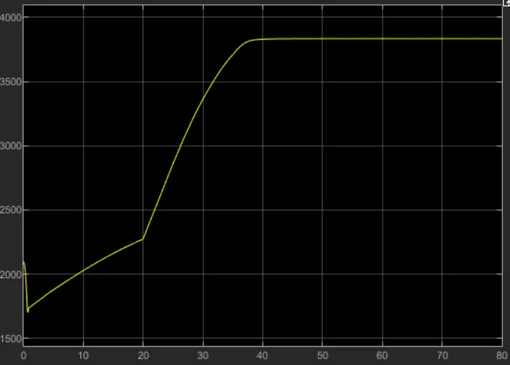
From the above plot we can observe that when Break input is 0 and Throttle input is 0.3 for t=20sec then velocity will reach by 20km/hr. By increasing the Throttle input to 1, then the velocity value will increase and reaches to maximum velocity.

The following daigram shows the Engine torque-speed curve. Which is inputted to the generic engine block to generate output RPM accordingly.

The image which is shown below indicates the Engine speed plot. Engine speed will decrease at the begining because of increasing gear ratio. which increases the torque by increasing the throttle input to 1, then engine speed value will increase and it reaches to the maximun speed.

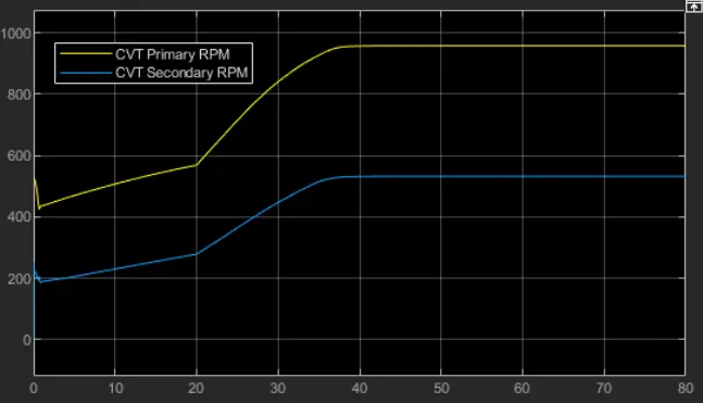
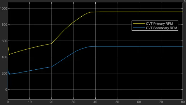
The following figure shows that the CVT shaft speed of Primary and Secondary RPM. As we discussed before when the variator which is connected to primary pulley goes inward then the variator of secondary pulley goes outward. Then the Primary RPM is greater than the Secondary RPM. Which is observed through the following plot.

Model of BAJA ATV with Dashboard:

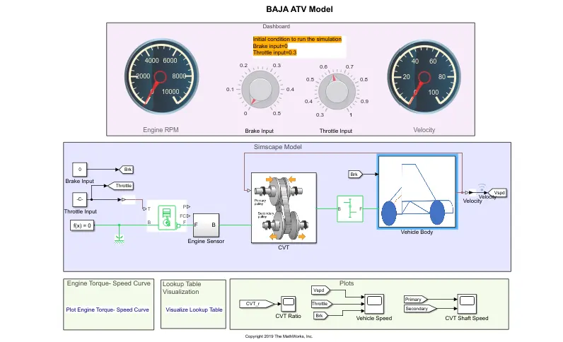
The following daigram shows the simulink model of BAJA ATV with Dashboard is shown in the following figure.

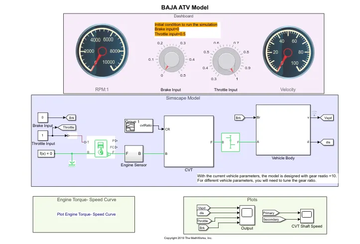
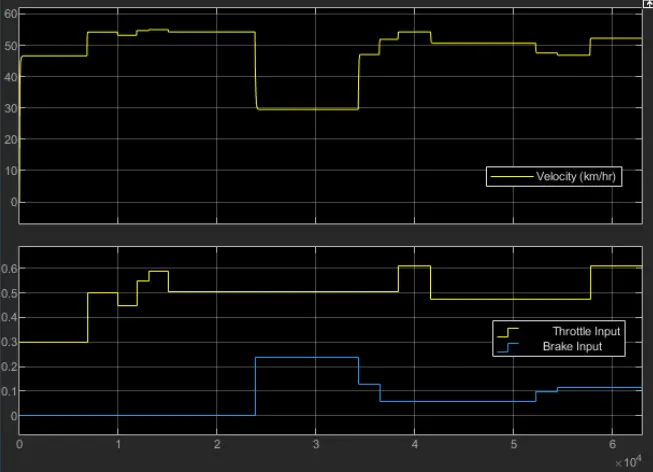
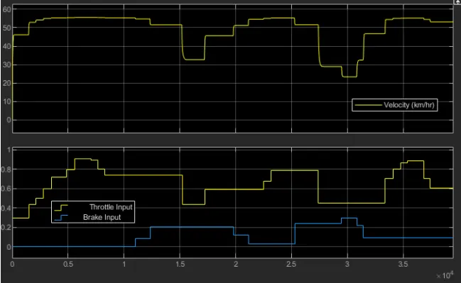
In this plot the break and throttle inputs are given through the Dashboard. We can observer from the above daigram the Dashboard shows all the blocks which are, RPM meter, Break input, Throttle input and velocity gauge from there we can directly control the inputs and obseve the changes in velocity according to the speeds. Intially the RPM and Velocity are at 0RPM and 0 km/hr. Where we can manually change the values of break an throttke so by varying the different values we can observe the velocity plot. The following figure shows the velociity plot according to the given throttle and break inputs. We can observe that there is no proper graph because of continuous varying in the inputs.

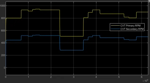
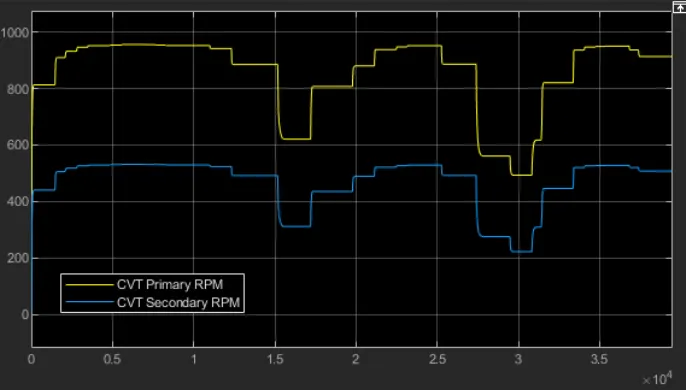
The following daigram shows the shaft speeds of the two pulleys. As we know that the speed of primary pulley is greater than the speed of the secondary pulley foer the condition we are observing. And by increasing the break input value the speed value will decreases. Which is also can observe in the following figure.

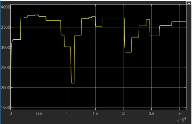
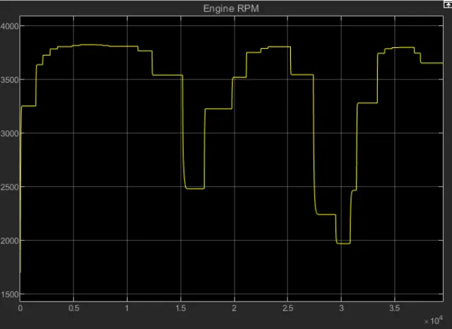
The image shows below represents the engine plot. By increasing the throttle input value it will increase the engine speed, and by increasing the brake input value it will decreases the engine speed. Accordingly following plot has been observed.

Model2 of BAJA ATV:

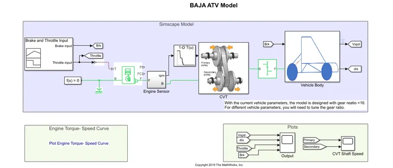
The following image shows that the closed loop model of the BAJA ATV. There is a feedback from the output to input as we can see in the following figure. In addition to the previous model wil add a Look up table. The workup process and construction is same as the previous except the lookup table.

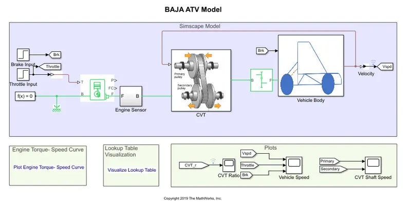
The following image shows the BAJA ATV model with look up table block. Here we are using 2-D Lookup table instead of Signal builder block for CVT ratio. The interpolation and extrapolation methods are set to linear.

In this model the inner part of the CVT block is shown in the following image.

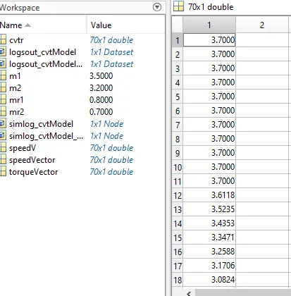
By using the workspace will enter the all data related to Lookup table. Will add the cvt ratios and speed values through in to the lookup table. The following images shows the data we are adding in the workspace.

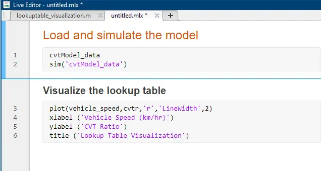
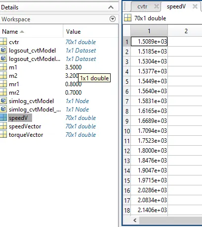
Right click on the Lookup table block and choose Foundation library option and then Plot option to visualize the Lookup table. The following images shows the Look table visualization.

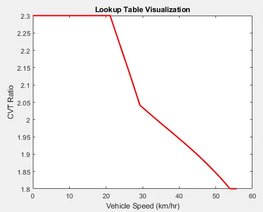
The following plot shows the values of Lookup table input data given to CVT.

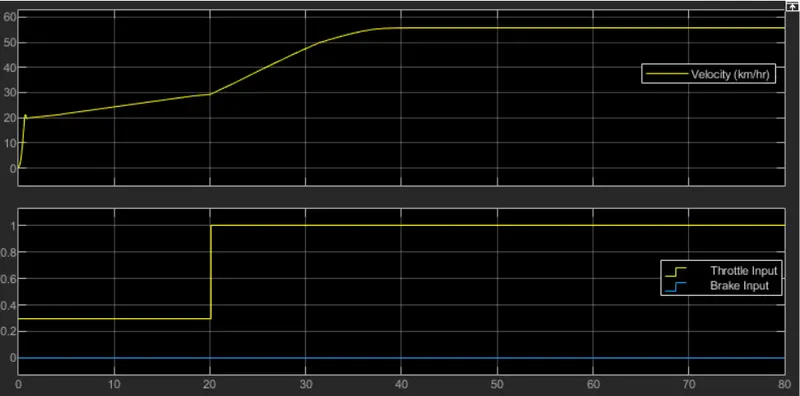
Same as the previous model here the value of throttle signal will be set to a value and by applying the lookup table table data will get the following output velocity. the velocity will reach maximum value when throttle value is more than 1.

The following plots shows the CVT shaft ratios of primary and secondary pulley. As we know Rp is greater than Rs.

And in the other case will use Dashboard to control the input values. Where we can directly control the velocity by changing the RPM values through break and throttle inputs. The following image shows the model of BAJA ATV with Dashboard.

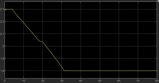
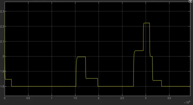
The following diagram will shows the CVT ration plot from the Lookup table data. From the following plot we can say that CVT ratio will vary by changing the throttle gauge. If throttle value increases CVT ratio decreases and vice versa.

The folowing image shows the vechile speed plot. This output plkot can be taken by varying the throttle and break inputs manually from the dasboard. From this plot we can say that by increasing the break input value its velocity decreases and if it decreases velocity value will increases.

The following image shows the shaft ratios of the CVT primary and secondary pulley. We are varying the values continuously so that is why the plot is not in a defined path but we can observe that as per our data Rp>Rs.

The following daigram represents the Engine speed plot. It can be observed that by increasing the throttle input value engine speed is increasing and by increasing the brake input value it will decrese the engine speed. and vice versa.

Conclusion:

System level simulation of BAJA All Terrain Vechile with different models in different cases has been studied. Technical report for the model has been prepared and output results are plottled.

Simulink model:

https://www.mathworks.com/matlabcentral/fileexchange/70576-baja-all-terrain-vehicle-atv-model

I have uploaded direct link to the simulink models. if it is required i will attach each simulink model.