Week 7 State of charge estimation

Q) Simulate the 3 test cases from the harness dashboard and write a detailed report on the results?

ANS:

TEST CASE 1:

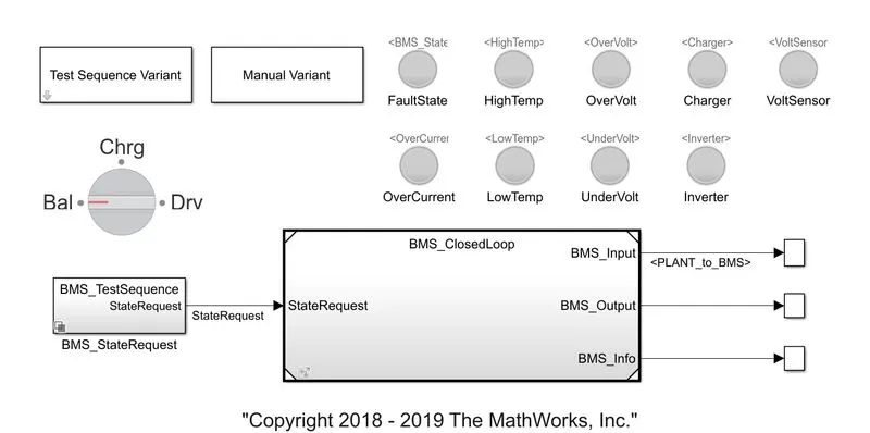
Now we set the Test Sequence Variant to 1.

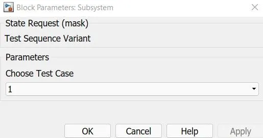
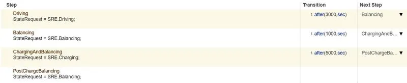
Now run the Simulink and plotted the graphs:

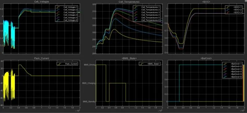
• The principal diagram demonstrates the cell voltage of the relative multitude of cells engaged with the battery pack we originally saw that cell voltages change as the current streams in and out. toward the start of the reenactment, the voltages are marginally unique since we introduce the model with a slight partner of unevenness the voltages are redirected from the scope of 3.1 v to 3.9 volts for the time-frame of 0.3*10^4 sec, and afterwards, there is an equilibriums condition of all voltage of their particular cells and afterwards, there is an abrupt climb in cell voltage till they arrive at 4.2 volts and toward the finish of the reproduction, the qualities merge towards each other and attempting to adjust the voltages till the end still there is a little distinction in their voltages and the voltage line streams between 4 to 4.2 volt. since the framework goes on backup mode.
• In charging state during the consistent current stage current(current is avoiding in the scope of 19 A TO - 70 for 0.3*10^4 sec) is discussed since the most extreme cell voltage is high, enough contrasted with recommended 4.4-volt limit that an exorbitantly high current control the voltage past the edge essentially restricting the existence of the battery.
• The temperature (it's beginning from the scope of 289-degree Celcius and toward the end, every one of the cells has an alternate temperature) follows to show the huge inconsistency between the most sweltering and coldest cell the explanation is basically a result of balance in the consolidation layer as far as warm conduct. Cell no 6 is essentially more sweltering the phone no 1 since it is thermally protected on one side. regardless of whether the most extreme temperature came to during the reenactment isn't worried as far as security. the temperature distinction at cell no 6 at its higher temperature will ultimately cost a lot quicker debasement of cell 6 contrasted with cell 1 prompting bothersome and unevenness in cell condition. hence need a functioning warm administration framework to keep warm contrasts inside a couple of degrees Celcius.
• Chart no 3 show the soc of three unique battery cell each performed with various matter yellow relates to section counting, blue relates to ukf and orange to ekf, the underlying soc is 75%, notwithstanding, the recreation so appraises need to instate it to 80% to set their ability to recuperate it is evident that coulomb counting never does on the grounds that it has no real way to acknowledge it is off-base because of the shortfall of voltage data. both normal channel calculations then again recuperate from the underlying mistake inside the main hour of reenacted time. With the ekf marginally beating then ukf.

TEST CASE 2:

Now we set the Test Sequence Variant to 2.

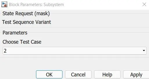
Now run the Simulink and plotted the graphs:

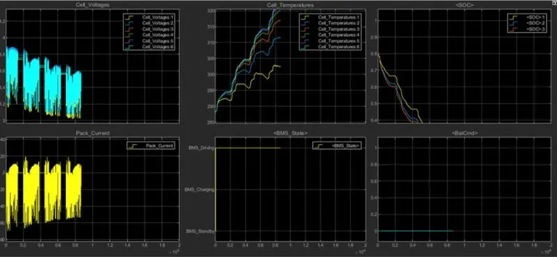
• In the underlying state, the voltage of the relative multitude of cells are diverting in a similar way and dropping somewhat in the scope of 3 to 3.9 volt it has 4 vacillation zones and in the middle of every one of these fluctuating zone, they are steady for while and this stage goes on for 0.85*10^4 sec. (all through the reproduction BMS has placed on driving mode).

• Then again the current diagram has precisely streamed in a similar way yet the other way when voltage is getting drop current required is high and current streams in the scope of - 70 A to 20 A.

• The temperature of the relative multitude of cells starts from 288-degree Celcius and they get dissipated every one of the cells has an alternate temperature) follows show the huge inconsistency between the most sweltering and coldest cell the explanation is basically a result of evenness in the consolidation layer in terms of warm conduct. cell no 6 is essentially more sizzling the cell no 1 since it is thermally protected on one side. regardless of whether the most extreme temperature came to during the reproduction isn't worried as far as security.

• The cells are at first at 80% of soc and afterwards, they're falling at various time spans. to set their capacity to recover.it is obvious that coulomb counting never does on the grounds that it has no real way to acknowledge it is off-base because of the shortfall of voltage data. both normal channel calculations then again recuperate from the underlying blunder inside the principal hour of reenacted time. with the ekf marginally beating then, at that point,
  ukf then is obvious that coulomb counting never does in light of the fact that it has no real way to acknowledge it isn't right because of the shortfall of voltage data. Both normal channel calculations then again recuperate from beginning mistake inside the main hour of reenacted time. with the mythical being somewhat outflanking the ukf.

• Different degrees demonstrate the bs state at every one of the equilibrium order flags separately. where it's on driving mode and order signals on zero lines.

TEST CASE 3:

Now we set the Test Sequence Variant to 3.

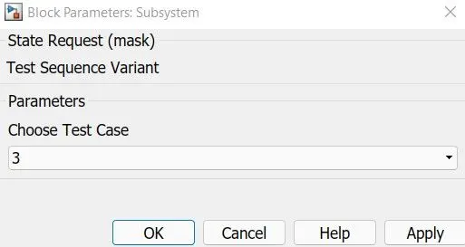
Now run the Simulink and plotted the graphs:

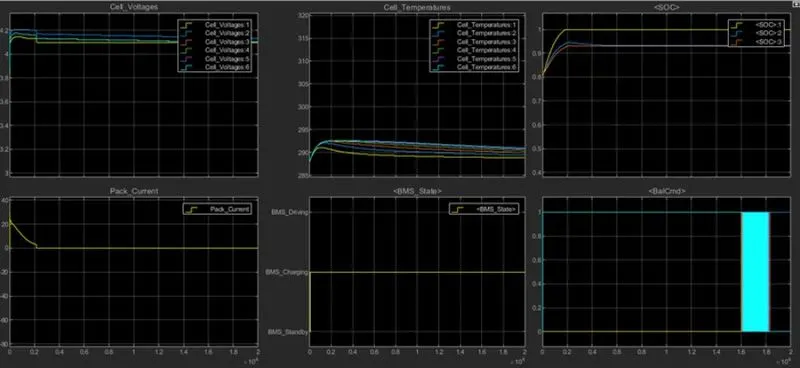
• every one of the cells is started at various voltages where the 6 is the one having the higher voltage of 4.2 volts and the first one has close around 4.1 v and staying falling under this range BMS on charging state all through the reenactment. so the voltage diagram move along in a straight line in light of the fact that the voltage supply goes on there has some diversion of voltage lines of various cells yet that is an exceptionally less measure of progress in voltage toward the finish of the reproduction BMS attempting to adjust the voltage definitely.
• The battery pack current is started with 20 An and afterwards, it tumbles to no current till its finished reenactment season of 0.2"10^4 sec and afterwards, it keeps up with the consistent current since it is placed on charging state and it stays steady all through the reenactment.
• All the cells start with 287-degree Celcius and afterwards every one of the cells keeps up with the straight line yet with various temperatures range. the end every one of the cells has an alternate temperature) follows show the huge disparity between the most sweltering and coldest cell the explanation is chiefly due to evenness in the consolidation layer as far as warm conduct. cell no 6 is all together more sultry the cell no 1 since it is thermally protected on one side. regardless of whether the greatest temperature came to during the reproduction isn't worried as far as security. the temperature distinction at cell no 6 at its higher temperature will ultimately cost a lot quicker corruption of cell 6 contrasted with cell 1 driving to unfortunate and lopsidedness in cell condition. in this manner need a functioning warm administration framework to keep warm contrasts inside a scarcely any degree Celcius.
• The soc is starting soc of three unique cells is at 80% as the. as the framework is placed on charging state the soc climbs up to 100 per cent for the yellow cell,ukf and ekf at first having different charging rates however after 0.4*10^4 sec they having an equivalent condition of charge of 91% and it keeps up with all through the reenactment .t is clear that coulomb counting never does on the grounds that it has no real way to acknowledge it is off-base because of the shortfall of voltage data. both normal channel calculations then again recuperate from the underlying mistake. ekf and urf marginally beating then, at that point, coulomb counting.
• Different degrees show the BMS state at every one of the equilibrium order flags separately. BMS on charging state and battery order passing sign between O to 1.

Q)What is coulomb counting? Refer to the above model and explain how BMS implements coulomb counting for SOC estimation?

ANS:

Coulomb counting is a technique used to track the State of Charge of a battery pack. It works by integrating the active flowing current (measured in amps) over time to derive the total sum of energy entering or leaving the battery pack. This produces a capacity that is typically measured in Amp-hours.

The ‘coulomb counting’ or CoulCount method was developed by Schmitt et al. as a heuristic method, although the underlying theory is reasonably accessible. It depends on the recording of the current noise only. The signal is filtered with a high-pass filter with a cut-off frequency of 0.01 Hz. The filter may be either analogue (although the implementation of a good-quality 0.01 Hz analogue filter is difficult) or digital. The absolute value of the measured current samples is then summed over time. A steep slope is taken as an indication of rapid corrosion, although it is not possible to calibrate this in terms of an estimated corrosion rate.

It can be shown that this method is similar to integrating the standard deviation of current over time. The use of the integrating plot provides a form of low pass filtering that may make it easier to see trends, but this can also be accomplished by digital filtering. The use of only the current noise restricts the value of the technique, as it does not allow for the estimation of the noise resistance (and hence the corrosion rate), and it is difficult to see what real advantages the method has over the conventional three-electrode method, although the use of integrating plots may be of value.

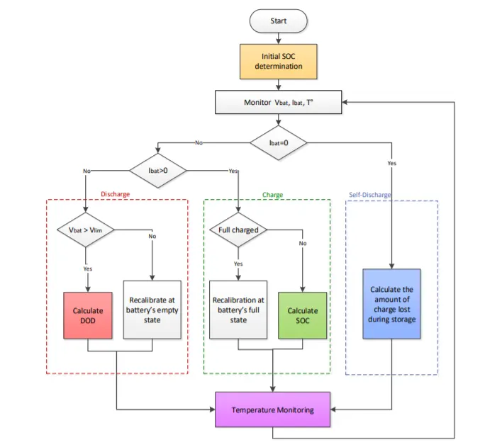
The flow chart of Coulomb Counting:

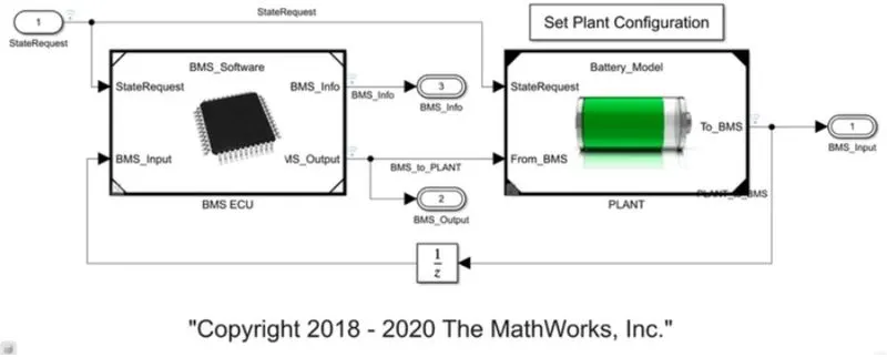
• This model contains BMS ECU and PLANT to ascertain gauge soc of battery the board framework we want to enter the plant block.

• Before we charge our vehicle we really want a precise Estimation of battery SOC, in the battery framework, we don't quantify the condition of charge we measure various things like battery pack current cell voltage and cell voltage which we accept signs as contribution from the plant.

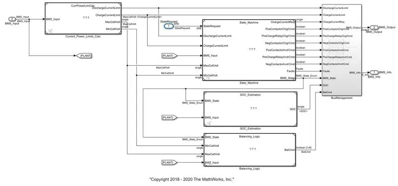
• Subsequent to entering the plant block we can see the state machine, SOC assessment, and adjusting rationale block.

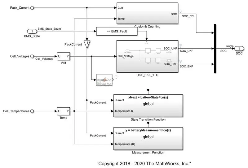
• In which we going to concentrate on SOC assessment. In this SOC assessment block, we can see three distinct procedures for the condition of charge assessment. Every one of the three strategies has its own benefits and restrictions. The primary strategy is coulomb counting and the other two are unscented(ukf) and expanded Kalman filter(ekf). Here we are worried about the coulomb counting technique.

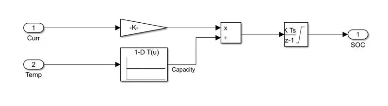
• In coulomb counting technique block. It takes two info signals, for example, current and temp and the current sign goes to acquire block and the temp signal goes to query tables of battery time and current, and both the squares are associated with the separated square and these signs are associated with the discrete-time integrator to follow the charge and which at long last assists with computing the condition of charge.

• Which comprise of coordinating a current and doesn't leave the cell for that here we utilise discrete-time integrator to give the track of the cell charge of the time the advantages of this is its effortlessness and its low capitation cost and the downsides are an aggregation of current sensor mistake and its failure to recuperate from some unacceptable introductory condition. From the absence of criticism from voltage estimations.