Project 2 - Rankine cycle Simulator
Rankine Cycle Simulator
Working Theory of a Rankine Cycle Simulator:
The Rankine cycle or Rankine Vapor Cycle is the interaction broadly utilized by power plants, for example, coal-terminated power plants or atomic reactors. In this instrument, fuel is used to create heat inside a boiler, changing over water into steam which then, at that point, extends through a turbine delivering valuable work. This cycle was created in 1859 by Scottish specialist William J.M. Rankine. Rankine Cycle is a thermodynamic cycle that converts heat into mechanical energy—which for the most part gets changed into power by electrical age.
- Pump: Compression of the fluid to high pressure using a pump (this takes work). (Figure 2: Steps 3 to 4)
- Boiler: The compressed fluid is heated to the final temperature (at boiling point). Therefore, a phase change occurs—from liquid to vapor. (Figure 2: Steps 4 to 1)
- Turbine: Expansion of the vapor in the turbine. (Figure 2: Steps 1 to 2)
- Condenser: Condensation of the vapor in the condenser (where the waste heat goes to the final heat sink (the atmosphere or a large body of water (ex. lake or river). (Figure 2: Steps 2 to 3)
- Isentropic expansion - steam enters the turbine where it is expanded bo pressure, and temperature will decrease. The turbine generates electricity.
- Constant pressure heat rejection - the wet steam rejects heat into the condenser, where Its phase changes again and becomes saturated liquid.
- Isentropic compression - water is pumped from low pressure to high pressure isentropically. The pump requires some input it.
- Constant pressure heat addition - water enters the boiler, heated until its phase change is dry saturated vapor. The process takes place under constant pressure, and heat is added to water. That's why it is called constant pressure heat addition.
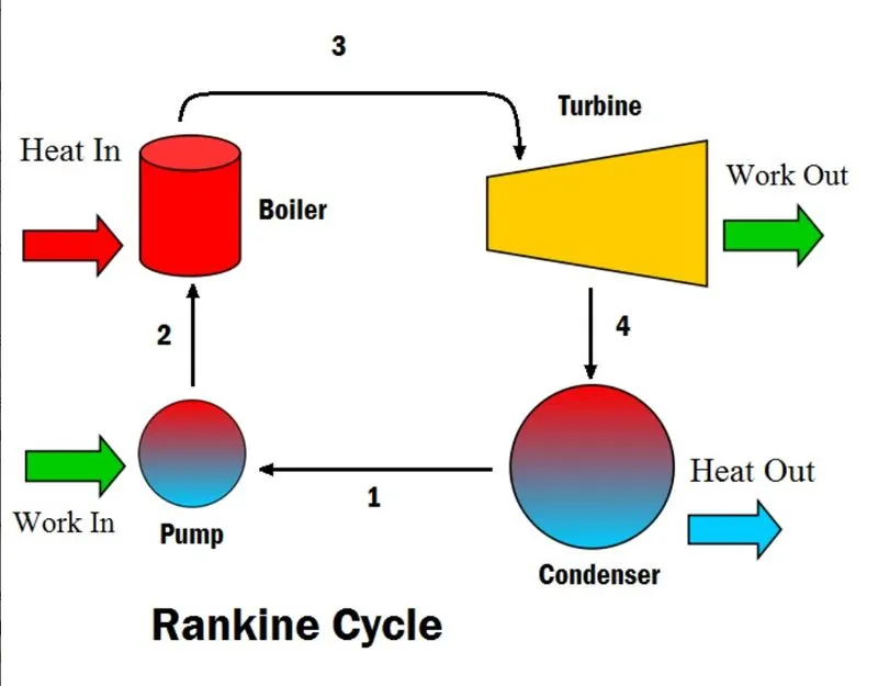
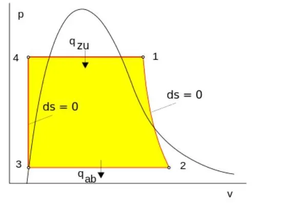
FIGURE 1: A simple schematic with components for the Rankine Cycle. Figure 2. The pressure-volume diagram of the Rankine cycle. This illustrates the changes in pressure and volume the working fluid (water) undergoes to produce work.
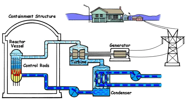
Figure 3. Rankine cycle in a nuclear power plant.
Explanation of the code:
- First, using the disp command, we display the Rankine Cycle Simulator and all four processes.
- Next, assign the given parameters for pressures and temperature.
- Next, XSteam data is used to extract steam and water properties of enthalpy, entropy at specific pressure and temperatures for saturated liquid, saturated vapor conditions.
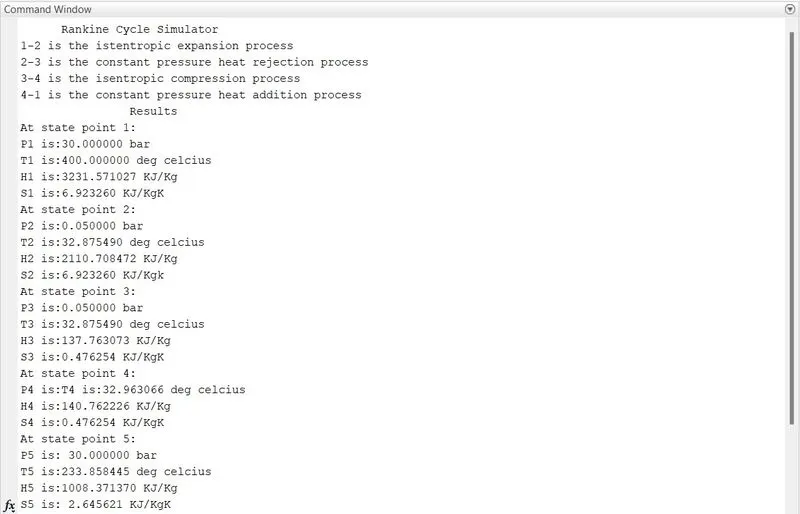
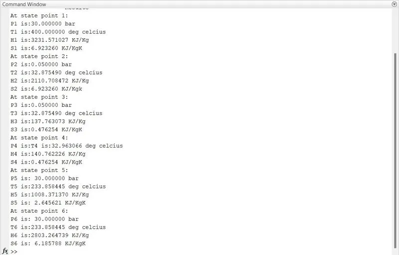
- Next, using the fprintf command, print all the values of their respective variables. Do the same process for all the stages to find the unknowns.
- Next, using the for loop command, extract the entropy and enthalpy values and save them into variables.
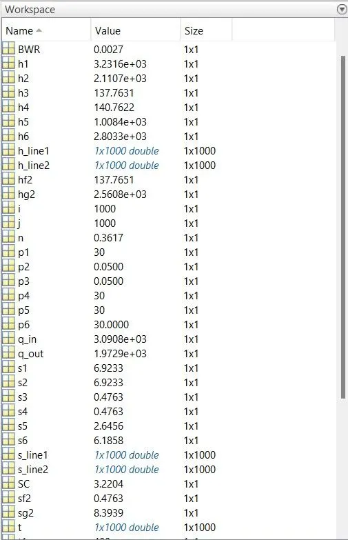
- Next, calculate the work output and back water ratio (BWR).
- Next, plot the graphs T-S and H-S with all the available values.
- Next, plot the saturation lines on the T-S and H-S graphs.
close all
clear all
clc

%Displaying Rankine Cycle Simulator and its processess

disp('      Rankine Cycle Simulator')
disp('1-2 is the istentropic expansion process')
disp('2-3 is the constant pressure heat rejection process')
disp('3-4 is the isentropic compression process')
disp('4-1 is the constant pressure heat addition process')

%Variables for stage1

p1 = 30;
t1 = 400;
h1 = XSteam('h_pt',30,400);
s1 = XSteam('s_ph',30,h1);
fprintf('                Results \n')
fprintf('At state point 1: \n')
fprintf('P1 is:%f bar \n',p1)
fprintf('T1 is:%f deg celcius \n',t1)
fprintf('H1 is:%f KJ/Kg \n',h1)
fprintf('S1 is:%f KJ/KgK \n',s1)

%Variables for stage2

p2 = 0.05;
s2 = s1;
t2 = XSteam('T_ps',0.05,6.1858);
sf2 = XSteam('sL_p',p2);
sg2 = XSteam('sV_p',p2);
hf2 = XSteam('hL_p',p2);
hg2 = XSteam('hV_p',p2);
x = ((s2 - sf2)/(sg2 - sf2));
h2 = hf2 + (x*(hg2 - hf2));
V2 = XSteam ('v_ph',p2,h2);
fprintf ('At state point 2: \n')
fprintf('P2 is:%f bar \n',p2)
fprintf ('T2 is:%f deg celcius \n',t2)
fprintf('H2 is:%f KJ/Kg \n',h2)
fprintf('S2 is:%f KJ/Kgk \n',s2)

% variables for stage3

t3 = t2;
p3 = p2;
s3 = XSteam('sL_p',p3);
h3 = XSteam('hL_T',32.875);
v3 = XSteam('v_ph',p3,h3);
fprintf('At state point 3: \n')
fprintf('P3 is:%f bar \n',p3)
fprintf('T3 is:%f deg celcius \n',t3)
fprintf('H3 is:%f KJ/Kg \n',h3)
fprintf('S3 is:%f KJ/KgK \n',s3)

% variables for stage4

s4 = s3;
v4 = v3;
p4 = p1;
h4 = XSteam('h_ps',p4,s4);
t4 = XSteam ('T_hs',h4,s4) ;
fprintf('At state point 4: \n')
fprintf('P4 is:% bar \n',p4)
fprintf ('T4 is:%f deg celcius \n',t4)
fprintf('H4 is:%f KJ/Kg \n',h4)
fprintf('S4 is:%f KJ/KgK \n',s4)

% variables for stage5

p5 = p4;
t5 = XSteam('Tsat_p',p5);
h5 = XSteam('hL_T',t5);
s5 = XSteam('sL_p',p5);
fprintf ('At state point 5: \n')
fprintf('P5 is: %f bar \n',p5)
fprintf('T5 is:%f deg celcius \n',t5)
fprintf('H5 is:%f KJ/Kg \n',h5)
fprintf('S5 is: %f KJ/KgK \n',s5)

% variables for stage6

t6 = t5;
p6 = XSteam('psat_T',t5);
s6 = XSteam('sV_T',t6);
h6 = XSteam('hV_T',t6);
fprintf('At state point 6: \n')
fprintf('P6 is: %f bar \n',p6)
fprintf('T6 is:%f deg celcius \n',t6)
fprintf('H6 is:%f KJ/Kg \n',h6)
fprintf('S6 is: %f KJ/KgK \n',s6)

% loop to find variables on saturation lines

t = linspace(0,400,1000);
for i=1:length(t)
s_line1(i) = XSteam('sL_T',t(i));
end
for j=1:length(t)
s_line2(j) = XSteam('sV_T',t(j));
end
for i=1:length(t)
h_line1(i) = XSteam('hL_T',t(i));
end
for j=1:length(t)
h_line2(j) = XSteam('hV_T',t(j));
end

% net work output calculation

w_turbine = h1 - h2;
w_pump = h4 - h3;
work = w_turbine - w_pump;
q_in = h1 - h4;
q_out = h2 - h3;

% thermal efficiency

n = work/q_in;

%Back work ratio

BWR = w_pump/w_turbine;

% Specific steam consumption

SC = 3600/work;

%plotting T-s graph

figure(1)
hold on
plot([s_line1 s_line2],[t t])
plot([s1 s2 s3 s4 s5 s6 s1],[t1 t2 t3 t4 t5 t6 t1])
text(s1,t1,'1')
text(s2,t2,'2')
text(s3,t3,'3')
text(s4,t4,'4')
text(s5,t5,'5')
text(s6,t6,'6')
title("Rankine cycle T-S Diagram")
xlabel('Entropy (KJ/KgK)')
ylabel('Temperature(K)')
axis([0,8,0,450])

%plotting h-s graph

figure(2)
hold on
plot([s_line1 s_line2], [h_line1 h_line2])
plot([s1 s2 s3 s4 s5 s6 s1],[h1 h2 h3 h4 h5 h6 h1])
text(s1,h1,'1')
text(s2,h2,'2')
text(s3,h3,'3')
text(s4,h4,'4')
text(s5,h5,'5')
text(s6,h6,'6')
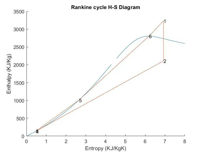
title("Rankine cycle H-S Diagram")
xlabel('Entropy (KJ/KgK)')
ylabel('Enthalpy (KJ/Kg)')
axis([0,8,0,3500])
OUTPUTS:
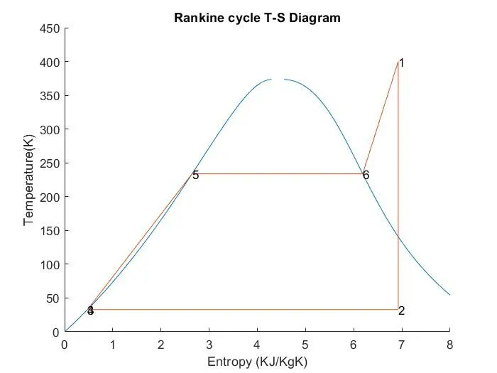
COMMAND WINDOWS:
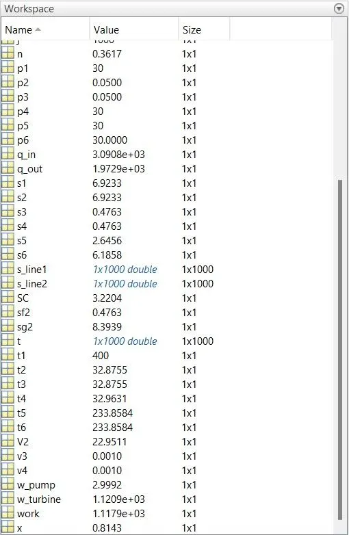
WORKSPACE WINDOWS:
REFERENCES: