Week 3 - Solving second order ODEs

In this challenge, we are doing the second-order ODE using a simple pendulum as an example:

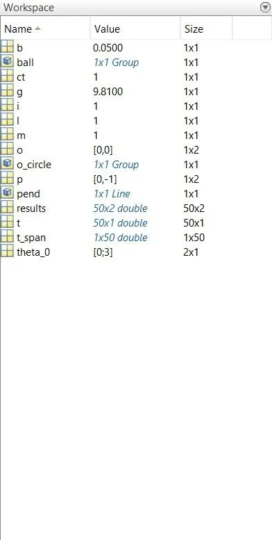
1. We have assumed the initial condition for the simple pendulum. L=1 metre, m=1 kg, b=0.05, g=9.81 m/s2. The pendulum's motion is for 20 secs, and the initial angular displacement and initial angular velocity are 0 and 3 rad/s.
2. So next, the time span is assumed from 0 to 20 secs with 50 intervals in between.
3. Next, I wrote an ode function to solve the second-order ODE. function [dtheta_dt] = ode_func(t,theta,b,g,l,m) ; theta1 = theta(1) ; theta2 = theta(2) ; dtheta1_dt = theta2 ; dtheta2_dt = (-b/m)*theta2 - (g/l)*sin(theta1) ; dtheta_dt = [dtheta1_dt; dtheta2_dt] ; end. In this function we have given the initial values and solve the second order ODE by splitting them into two parts.
4. Next, to solve the ODE I wrote the command [t results] = ode45(@(t,theta) ode_func(t, theta, b,g,l,m), t_span, theta_0); with all the conditions given.
5. Next, to animate the pendulum, I have assumed the origin for the pendulum. Then given the pendulum length measurements, ball measurement at the origin, and the other end of the pendulum.
6. Next, I gave a time interval for the loop. With a pause of 0.05, I gave limits to the axis. Then deleted all the items which were not in the final loop.

7. Next, we will get individual frames and save them in an array called M. Ct represents every frame.

8. After giving the frames, we are going to increase the counter.

9. Movie (M) means the MATLAB will generate a movie with all the frames in the array M.

10. Next, we will generate the animation video using the command videofile = VideoWriter('simple pendulum.avi');

11. Next, we will open the videofile, write the videofile with (videofile, M), and then close the videofile.

clear all;
close all;
clc;

%Initial Parameters of the pendulum
l = 1;
m = 1;
b = 0.05;
g = 9.81;


theta_0 = [0;3];

%time points
t_span = linspace (0,20,50);

%solve ODE
[t results] = ode45(@(t,theta) ode_func(t, theta, b,g,l,m), t_span, theta_0);

%Origin

o = [0 0];
ct = 1;

%loop for animation

for i = 1:length(t)
    %Mass Point
    p = l*[sin(results(i,1)) -cos(results(i,1))];
    
    %Circle in Origin
    o_circle = viscircles(o,0.01);
    %pendulum
    pend = line([o(1) p(1)],[o(2) p(2)]);
    %Ball
    ball = viscircles(p,0.05);
    
    %Time Interval to update the plot
    pause(0.05)
    axis([-1.5 1.5 -1.5 0])
    grid on
    xlabel('time')
    ylabel('plot')
    M(ct) = getframe(gcf);
    ct = ct+1;
       
    %Delete previous objects if it is not it the final loop
    
    if i<length(t)
        delete(pend);
        delete(ball);
        delete(o_circle);
    end   
end

videofile = VideoWriter('simple pendulum.avi');
open(videofile);
writeVideo(videofile,M)
close(videofile);

function [dtheta_dt] = ode_func(t,theta,b,g,l,m)
theta1 = theta(1)
theta2 = theta(2)
dtheta1_dt = theta2;
dtheta2_dt = (-b/m)*theta2 - (g/l)*sin(theta1);
dtheta_dt = [dtheta1_dt; dtheta2_dt];
end

https://youtu.be/DI70YJ2lxuM