Week 7 State of charge estimation

Week 7 Challenge : State of Charge Estimation

Q1.

https://in.mathworks.com/matlabcentral/fileexchange/72865-design-and-test-lithium-ion-battery-management-algorithms

Simulate the 3 test cases from harness dashboard and write a detailed report on the results.

Soln:

A battery management system (BMS) is said to be the brain of a battery pack. The BMS is an embedded system that monitors and manages all of the battery’s performance. Most importantly, it keeps the battery from operating outside of its safety margins. The battery management system is critical to the battery’s safe operation, overall performance, and longevity. Moreover, it protects whatever the lithium battery is installed in (EV, boat, RV etc.) and the people who are using it.

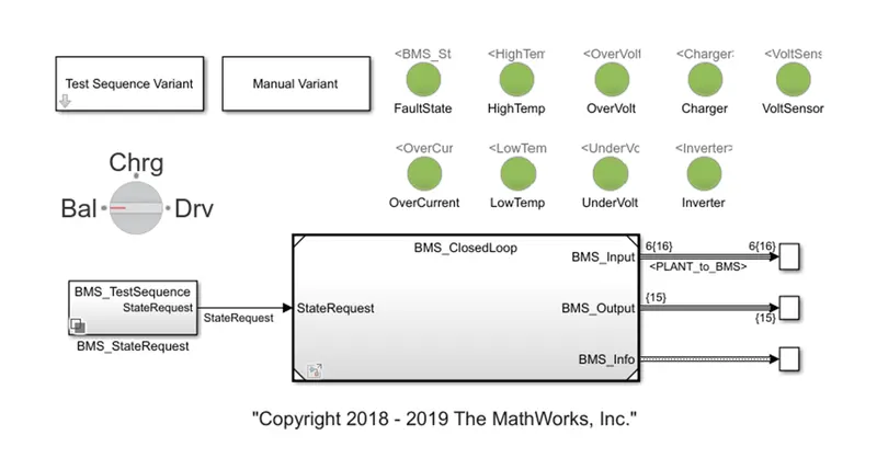
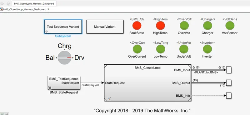
The model in the link above link gives a basic idea of a BMS system. It shows a how a BMS reacts and responds on occurring of any fault in the battery pack. The model indicates the user by glowing led in the dashboard. Using this model we can test battery packs for fault conditions and study the BMS response. The block diagram of the Test Harness is shown below.

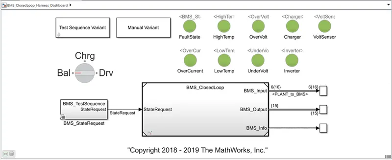
Inside this model , sits the main model of BMS. The figure is given below.

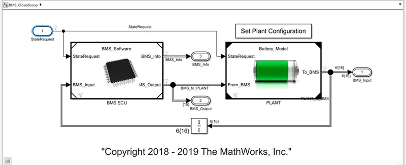
The BMS model mainly comprises of two components – BMS ECU and The Plant.

(a) BMS ECU: The BMS ECU is the heart of the system which controls all the program, control algorithm and logics.

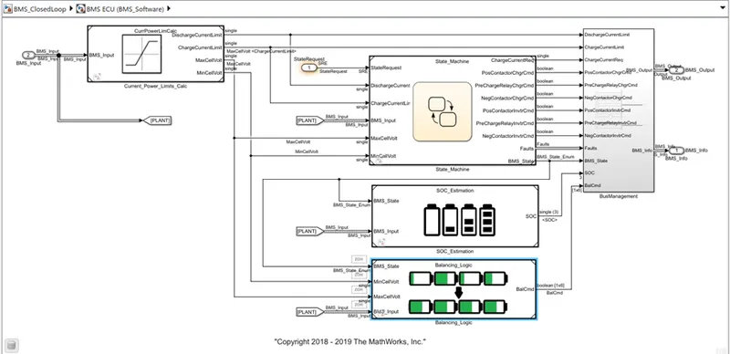
The BMS ECU unit comprises of the following subgraphs-

State_Machine; SOC_Estimation, Balancing _Logic, Current and Power Limit Calculation block and Bus management.

• The state machine implements processes of driving, charging and balancing.
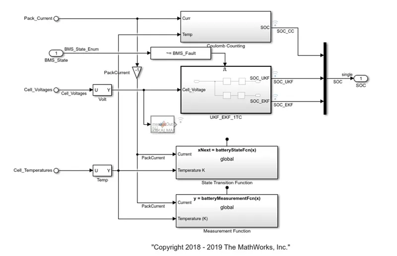
• The SoC estimation is a key element of a BMS ECU . It helps to estimate soc of the battery pack. In this model 3 different methods are used to calculate the SOC of the , they are- Coulomb Counting, Extended Kalman Filter and Unscented Kalman filter.

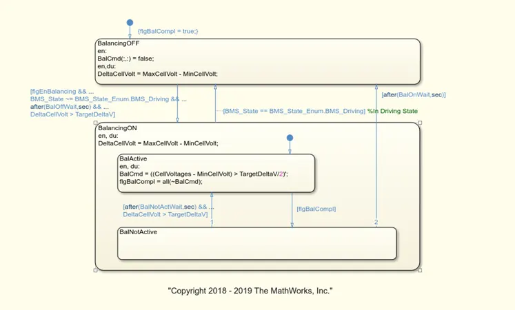
• The balancing logic block manages the battery pack while charging and discharging to remove any possibilities of occurrence of weak cell in the system. The cell balancing system continuously monitors and measures the voltage difference between the cells, and while the vehicle is not moving balancing of the cells happens if the voltage difference exceeds beyond threshold.

(b) Plant :

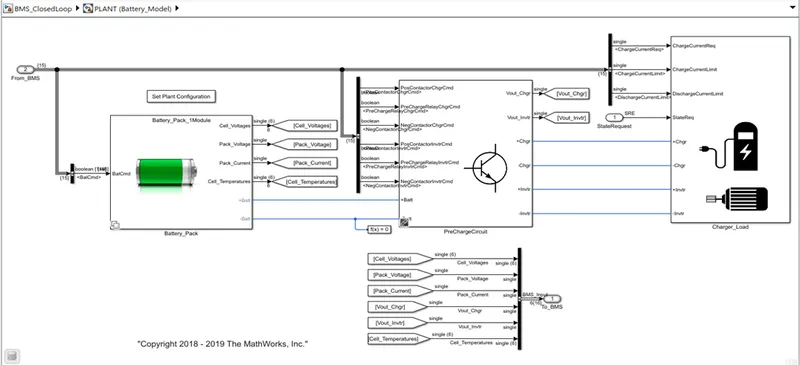
The plant model comprises of 3 main subsystems – Battery pack , Pre-charging Circuit and Charger Load.

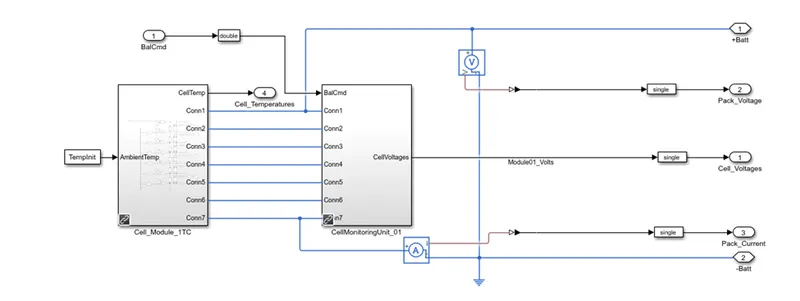
• The battery pack subsystem ,as the name suggests represents the battery pack made out of cells. Here 6 cells are combined in series to form a module. There is a option to choose 1 module or 16 modules to run the simulation. Voltmeter and ammeter are connected to monitor the voltage and current of the cells.

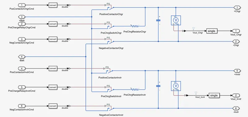
• Pre charge circuit is used to prevent the current rush while charging and discharging of battery pack and to avoid sparking in the contactors. A resistor connected in series to limit the current flow and a capacitor is connected to remove voltage ripple.

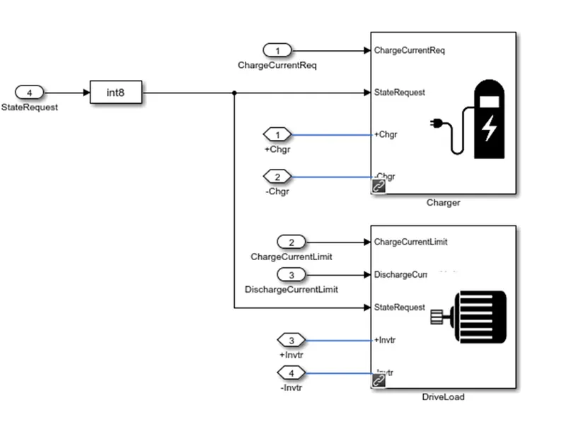
• The Charger Load subsystem applies charging or discharging based on the user input.

Simulation of Different Test Cases:

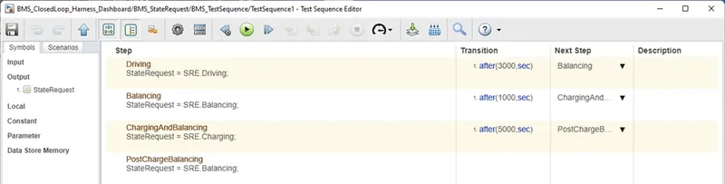
Using the Test harness dashboard 3 test case are simulated.

1. Test Case No 1:

The first test case simulation includes 3000 seconds in driving/discharge mode followed by 1000 seconds of standby mode then for 5000 seconds in charging and balancing mode and afterwards in the standby or balancing mode.

Results:

After running the simulation ,no fault is detected and dashboard LED’s are all green.

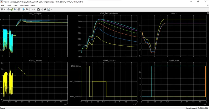
• The Cell Voltages plot displays the voltage of all 6 cells connected in series. In the first 3000 seconds the cell voltage decreases as it gets discharged. In the next 1000 seconds while the vehicle in stand by mode , the voltages are stabilized and cell balancing is done. In the charging period voltage again increases and shortly after it cell balancing is done, which stabilizes the voltage.
• The Pack_Current plot represents the current drawn from and given to the batteries during discharging and charging process. It is observed while charging , first it charges in constant current mode and then it charges in constant voltage mode.
• The Cell temperature plot gives the variation temperature of all cells for the simulation period. It can be noticed that temperature rises on charging and discharging of cells.
• The SOC plot shows the SOC of the battery module during the test period. SOC is calculated in 3 different methods so we observe 3 lines in the soc plot. The yellow line is for Coulomb counting, blue line for UKF and red is EKF method of SOC estimation. At the beginning of testing , the soc is around at 80% . After the driving process is completed , SOC dropped on to 40-50% In the standby period , SOC is observed to be constant. At 4000 seconds, the charging and balancing process starts and the SOC rises to 100% or close to 100% (ukf & ekf).
• The Next plot is the BMS State plot. This plot shows the various states of the BMS system over the test period which are driving, charging and standby.
• The last plot is the Balance Command plot for all the six cells. The first cell in the series will have the lowest voltage , so there is no balancing signal for cell one and we got 0 amplitude balancing

Curve in the output. However the other 5 cells are needed to be balanced with reference to the lowest cell so we see balancing command plot for other five cells. The balancing starts after the driving phase is over.

2. Test Case No 2:

In the second case, the simulation is bound for same 20000 seconds with first 10000 seconds of discharging phase followed by charging.

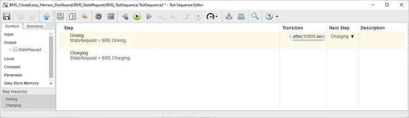
The model is run and here are the simulation output received.

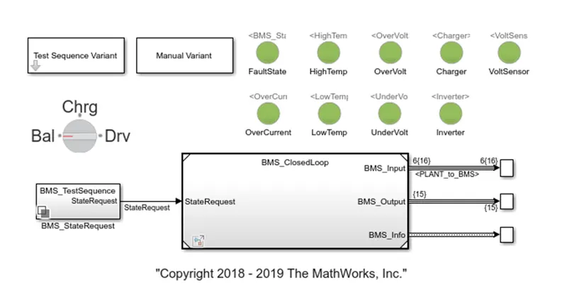
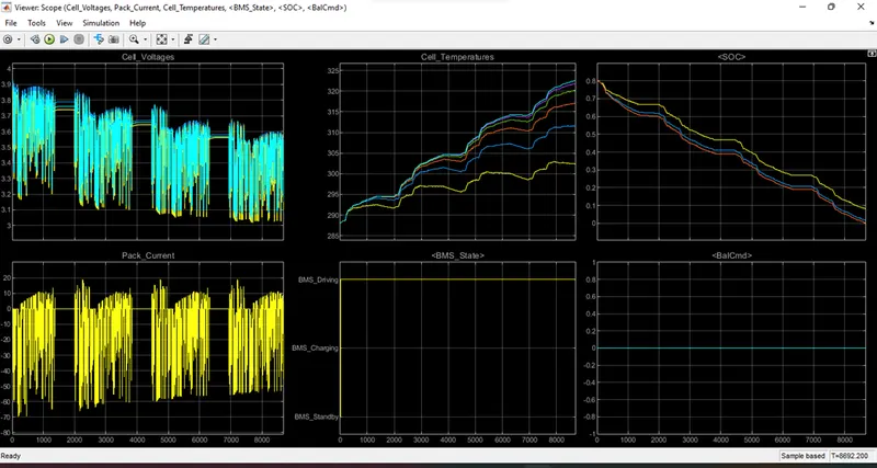
• The cell voltage plot shows the voltage levels of the 6 cells connected in series. The voltage keeps dropping after each drive cycle .After 8692 seconds voltage drops below the cut off threshold and simulation is stopped.
• The second plot is the peak current plot that gives the current variation of cells over time. It can be noticed that current variation sequence is repeated as time passes, since we are driving or discharging at same sequence for 10000 seconds. However, it cannot conclude the process.
• The third plot is the temperature plot. We can observe temperature of each cell is rising as time progresses. Because of the repeated discharge cycles cell temperatures increases from 287 K to 323 K .
• The SOC plot shows the SOC estimation by the three methods of calculation over time. The SOC of the battery module decreases with time as we keep repeating the discharge cycles. We started with 80% SOC , but before we can complete the driving phase , we hit 0% SOC at 8692 seconds.
• The next plot is the BMS State Plot. The plot only shows driving state as we didn’t get to move to the charging phase.
• The last plot is the cell balancing command plot. We didn’t any variation in this plot because during driving state cell balancing is not done.

3. Test Case No-3:

The condition for third test is we drive or discharge the battery for 5000 sec and then charge till the end of the simulation time of 20000 seconds.

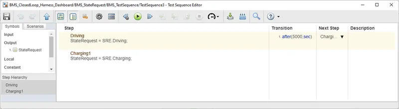
The model is run and the results are shown below.

• From the dashboard we can see fault occurring during time of simulation and it is a high temperature fault.

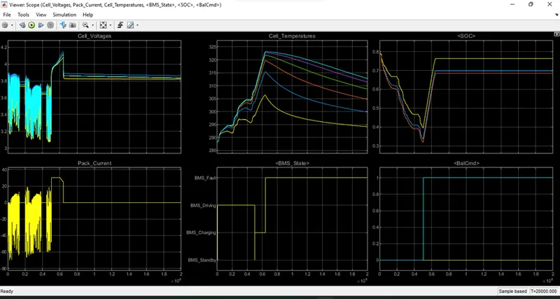
• The first plot with Cell Voltages displays the voltages of all 6 cells connected in the series. While the first 5000 seconds the voltage of the cells drops as the battery is discharging and then while charging the cell voltage increases and while the cell balancing the voltage stabilizes.
• The second plot with Pack_Current represents the current drawn and given to the battery while charging and discharging. It also seen that while charging, first the current remains constant, but then after 6600 secs, high temperature fault is detected and charging was abandoned.
• The third plots the cell temperature of all individual cells and we can see then while charging and discharging the cell temperature increases, at about 6600 seconds the cell temperature of the 6th cell increases to about 323.15 Kelvin, and the battery is sent to fault state.
• The fourth plot is the BMS state plot that shows the input state as per the given state input until the fault occurs at about 6600 seconds.
• The fifth plot shows the State of Charge of the entire pack by 3 different methods of calculation. The soc curve decreases as we discharge the battery and increases while charging. The battery is charged up to 70-75% and stops charging once the fault occurs.
• The sixth plot shows the cell balancing command for all six cells. The 1st cell is having the lowest voltage does not need balancing thus we can see that all the other cell's signal have a magnitude of 1 whereas the 1st cell signal is at zero magnitudes. The cell balancing starts when the battery starts to charge and at the onset of the fault the battery charging is stopped but the balancing happens.

Q2. What is coulomb counting? Refer to the above model and explain how BMS implements coulomb counting for SOC estimation?

Soln:

Coulomb counting is a technique used to track the state of charge of a battery pack. It works by integrating the active flowing current (measured in amps) over time to derive the total sum of energy entering or leaving the battery pack. This produces a capacity that is typically measured in Amp-hours.

The Coulomb counting method measures the discharging current of a battery and integrates the discharging current over time in order to estimate SOC. It is done to estimate the SOC(t), which is estimated from the discharging current, I(t), and previously estimated SOC values, SOC(t-1).

SOC is calculated by the following equation:

Where,

SOC(t) = State of charge at estimated time;

I(t) = Discharging current;

Q_N = Nominal battery capacity.

Implementation od coulomb counting for SOC estimation in the BMS model is done as below-

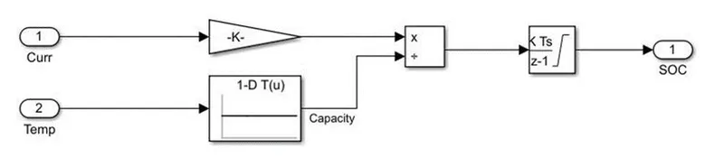
• The discharge current signal is converted from the physical system using a gain block.
• The gain block is integrated which gives us the discrete data.
• The temperature data is divided by using a lookup table with the discharge current rate.
• The output is then integrated with a discrete-time integrator block with a sample time of 0.1 sec to calculate the SOC of the battery pack.