Project

Aim : To carry out a system-level simulation of an Baja All-Terrain Vehicle.

Theory :

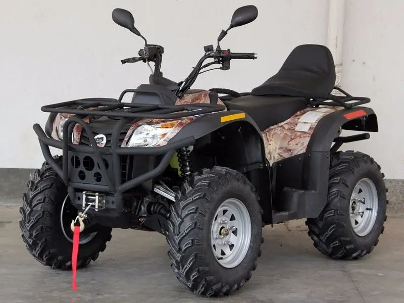
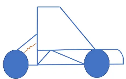
All terrain vehicle- An all-terrain vehicle (ATV), also known as a light utility vehicle (LUV), a quad bike, or simply a quad,

as defined by the American Nationaa Standards Institute (ANSI); is a vehicle that travels on low-pressure tires,with a seat

that is straddled by the operator, along with handlebars for steering control. As the name implies, itis designed to handle a

wider variety of terrain like sand, gravel, mud,ashphalt; than most other vehicles.

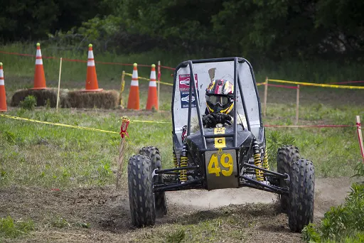
BAJA SAE - Baja SAE is an international competition run by the Society of Automotive Engineers (SAE International); that

challenges engineering students to design and build an off-road vehicle (ATV) that will survive the severe punishment of rough

terrain and in some competitions, water. As in real work situations, the engineers work together as a team to discover and

resolve technical challenges in design, test, and manufacturing. The most rugged of all the competitions, Baja SAE also gives

students the first-hand challenge of pursuing their passion while managing real-life demands and priorities. Each team's goal

is to design and build a prototype of an all-weather, rugged, single-seat, off-road recreational vehicle intended for sale to the

nonprofessional weekend off-road enthusiast.

Simulink Component :

Main components used-

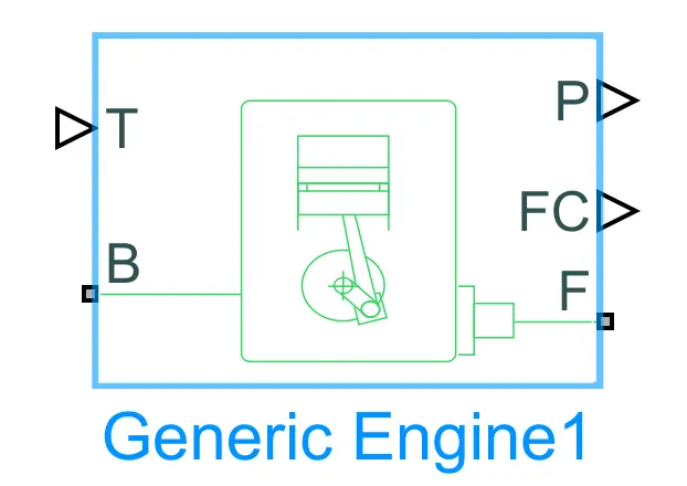
1. Generic Engine - The Generic Engine block represents a general internal combustion engine. This block is a suitable

generic engine for spark-ignition and diesel. Speed-power and speed-torque parameterizations are provided. A throttle

physical signal input specifies the normalized engine torque. Optional dynamic parameters include crankshaft inertia and

response time lag. A physical signal port outputs the engine fuel consumption rate based on the fuel consumption model

that you choose. Optional speed and redline controllers prevent engine stall and enable cruise control.

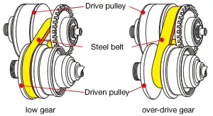
2. CVT- A continuously variable transmission (CVT) is an automatic transmission system that can change seamlessly through

a continuous range of gear ratios. To continuously vary its gear ratios, the CVT simultaneously adjusts the diameter of the

"drive pulley" that transmits torque from the engine and the "driven pulley" that transfers torque to the wheels. This contrasts

with other transmissions that provide a limited number of gear ratios in fixed steps. The flexibility of a CVT with suitable control

allows the engine to operate at a constant rpm while the vehicle moves at varying speeds. CVTs are used in automobiles, tractors,

snowmobiles and earthmoving equipments.

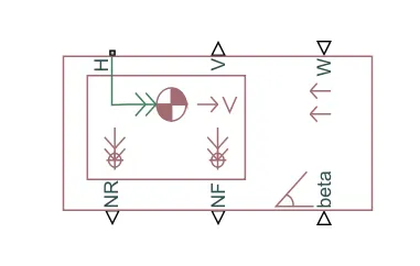
3. Vehicle body: Vehicle body is the main supporting structure of a vehicle, to which all other components are attached. In MATLAB,

the vehicle body block represents a two-axle vehicle body in longitudinal motion. The block accounts for body mass, aerodynamic drag,

road incline, and weight distribution between axles due to acceleration and road profile. The vehicle can have the same or a different

number of wheels on each axle. Optionally include pitch and suspension dynamics or additional variable mass and inertia. The vehicle

does not move vertically relative to the ground.

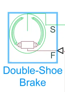
4. Double horse shoe brake- Represents a brake arranged as two pivoted rigid shoes symmetrically installed inside or outside a drum and

operated by one actuator. The actuator force causes the shoes to exert a friction torque on a shaft connected to the drum. Connection S is a

conserving rotational terminal associated with the drum shaft. Connection F is a physical signal port representing the force input to the actuator.

Positive force creates friction torque that resists shaft rotation. Optionally include thermal effects and expose thermal conserving port H by setting

Thermal port to Model.

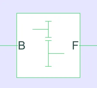
5. Simple gear - It represents a fixed-ratio gear or gear box. No inertia or compliance is modeled in this block; however, gear meshing and viscous

bearing losses can be optionally included.

Models :

A. Baja ATV model :-

The block diagram of the model is shown as follows-

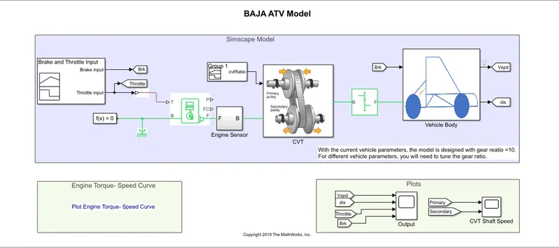
1. The input is given through a signal builder block. The brake and throttle are the input signal in this case. The brake is 0 and throttle is 0.6 for a time span of 80s.
2. The throttle signal is fed to the Generic Engine block.
3. The output of the engine block is fed to the cvt through a simple gear.
4. The cvt subgraph takes 2 inputs which are cvt ratio and the engine output. In the cvt subgraph, a variable ratio gear block is used and two inertia block is added on both sides of the gearbox. This setup represents the mechanical pulley cvt of real life.

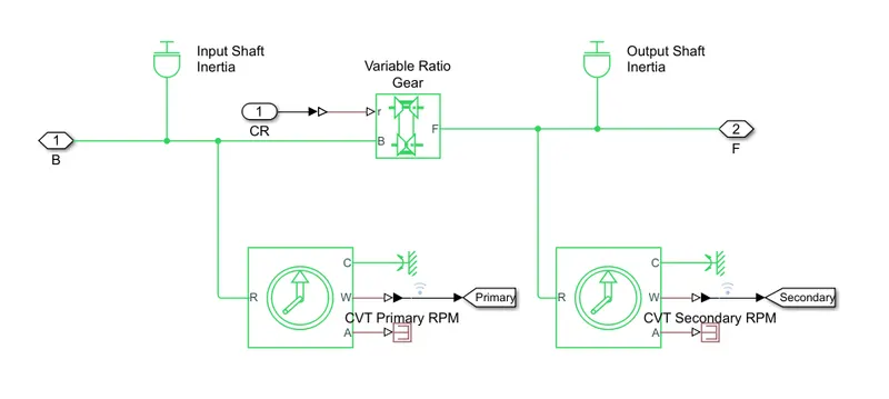
5. The output of the cvt subgraph is fed to the vehicle body via a simple gear. In the vehicle body subgraph, there’s a vehicle body block representing a two-axle vehicle

body in longitudinal motion ; connected to the four tires of the vehicle. The vehicle body accounts for the body mass, aerodynamic drag, road incline, and weight distribution

between axles due to acceleration and road profile. Connection H is the mechanical translational conserving port associated with the horizontal motion of the vehicle body. The

resulting traction motion developed by tires should be connected to this port. Connections V, NF, and NR are physical signal output ports for vehicle velocity and front and rear

normal wheel forces, respectively. Wheel forces are considered positive if acting downwards. Connections W and beta are physical signal input ports corresponding to headwind

speed and road inclination angle, respectively.

The parameters used for the vehicle body :-

Mass = 250 kg

No. of wheels per axle=2

Horizontal distance from cg to front axle= 1 m

Horizontal distance from cg to rear axle= 0.35 m

Cg height above ground= 0.7 m

Gravitational acceleration= 9.81 m/s^2

Drag co-efficient= 1.92

Frontal area= 0.735482 m^2

Air density=1.18 kg/m^3

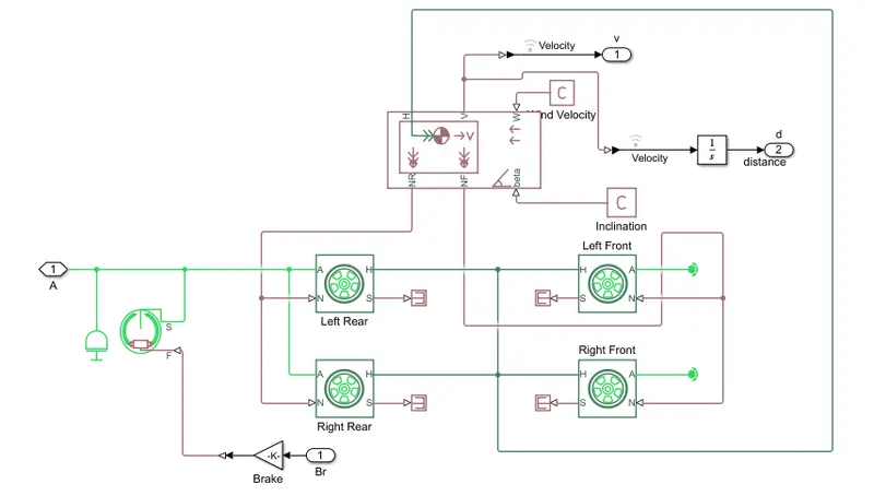
6. The input to vehicle body is first fed to the double horse-shoe brake an then the tires/wheels. It represents a brake arranged as two pivoted rigid shoes symmetrically

installed inside or outside a drum and operated by one actuator. The actuator force causes the shoes to exert a friction torque on a shaft connected to the drum. Default

Parameters are used for double horse-shoe brake and the tires are parameterized by Peak longitudinal force and corresponding slip.

Simulation Result:

The model is loaded in Simulink and run for a period of 200 seconds. The following results were found-

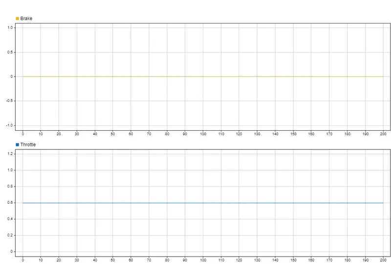
Inputs :

(i) Throttle and Brake input - Brake is set to 0 and the throttle input is set to 0.6 for the whole simulation time.

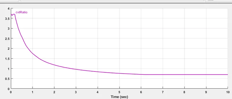
(ii) CVT Ratio : The input cvt ratio plot is as follows-

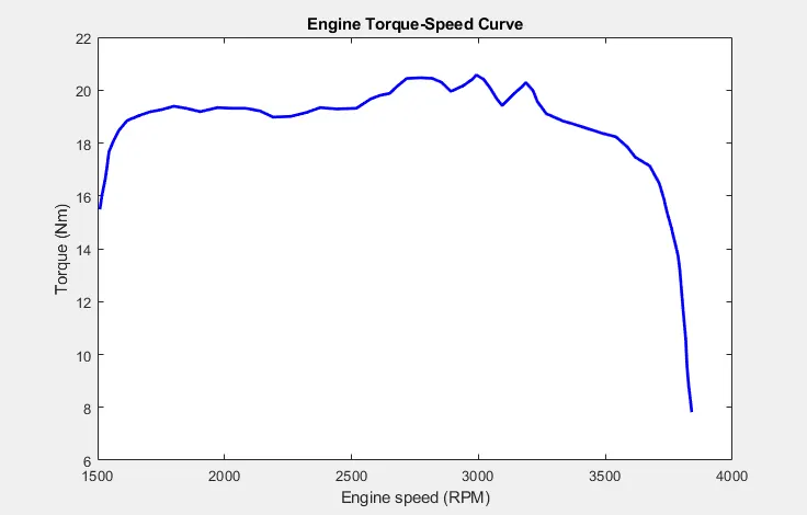
(iii) Engine Speed-Torque Characteristics : The speed-torque characteristics of the engine is given below-

Outputs :

After the simulation is completed we get the following output results-

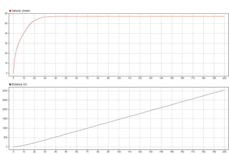
(i) Velocity-Distance Plot- At beginning velocity is 0 and as time passes it increases. After 20 seconds velocity exceeds 40 kmph. After 60 sec. velocity

reaches its peak value and stays there for the rest of simulation time. The distance travelled is also increases over time and reaches a final value of 2838.673 m

at the end of simulation.

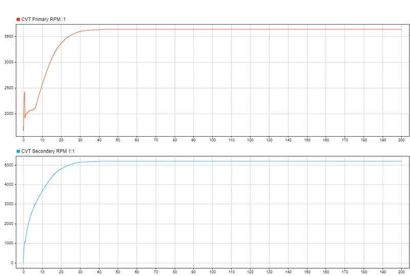
(ii) CVT RPM plot : The CVT primary and secondary rpm plot is acquired as below-

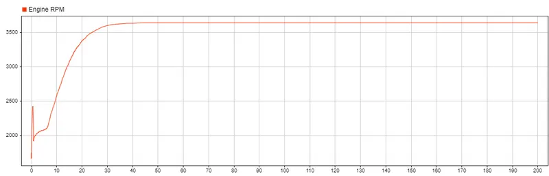
(iii) Engine RPM - The Engine RPM plot after completion of simulation is found as below-

B. BAJA ATV Model with Dashboard-

A Simulink model for BAJA ATV with dashboard arrangement is shown below. The model is same with previous one except the addition of a dashboard.

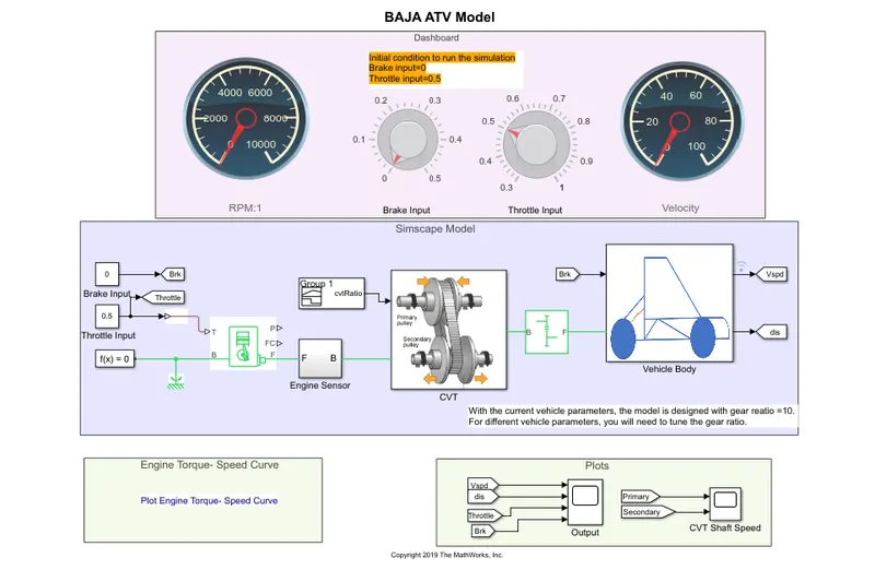
Dashboard- A dashboard is generally a control panel placed in front of the driver of the vehicle. It displays the instumentaton and control

of the vehicle. In Matlab also, we have dashboard block that let us do such things within a model. In this model, we are using dashboard to

display the engine rpm and velocity via gauges. Along with that , we have two knobs to control the brake and throttle input of the vehicle.

Simulation Results:

The initial condition of the model is set as

Brake input=0

Throttle input=0.5

The model is run for infinite simulation time and the inputs (throttle and brake) during the simulation. The change in engine rpm and velocity are observed

from the dashboard gauges. Plots are fetched from scope and data inspector.

Inputs:-

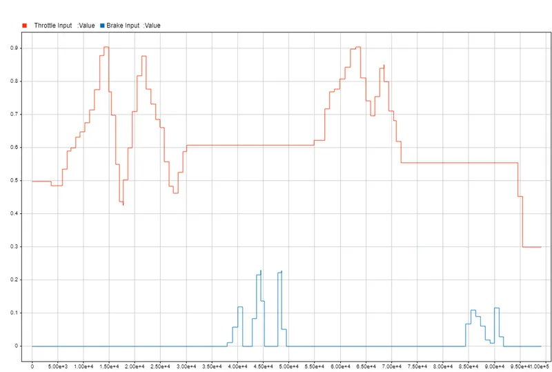
(i) Throttle and Brake : These inputs are varied during the simulation time.

(ii) CVT ratio: Cvt ratio is kept same as previous model.

Outputs:

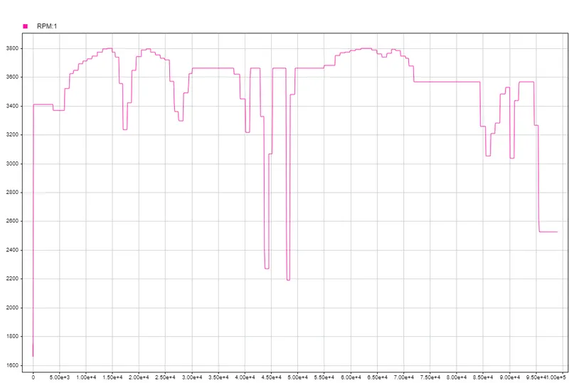
(i) Engine RPM: Following is the plot of the Engine RPM throughout the simulation time.

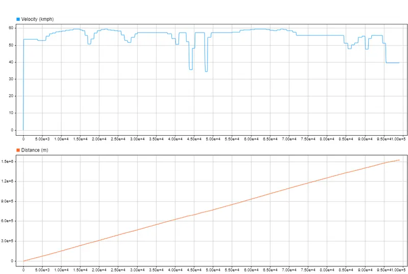
(ii) Velocity and Distance plot: The velocity and distance plot fetched from the scope and attached below. The velocity reaches to peak

value of 59 kmph.

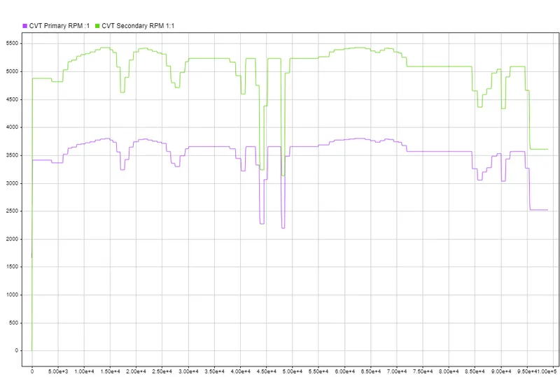
(iii) CVT RPM plot: The primary and secondary rpm of cvt is achieved as follows-

C. BAJA ATV Model with Lookup table-

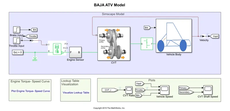
A simulink is model for Baja ATV model using lookup table is shown as below-

Lookup Table- A lookup table is an array of data that maps input values to output values, thereby approximating a mathematical function.

Given a set of input values, a lookup operation retrieves the corresponding output values from the table. If the lookup table does not explicitly

define the input values, Simulink can estimate an output value using interpolation, extrapolation, or rounding, where:

In real life the cvt ratio changes depending upon the velocity. That is why look up table is used here.This model is a close loop model. the data we are using

here for the lookup table is shown below,

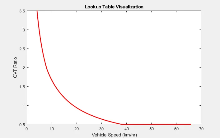
This data is fed to the variable ratio gear block in the cvt subgraph.

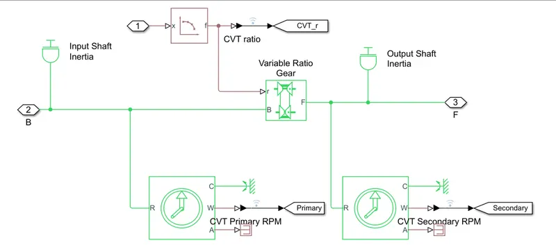
[fig.cvt subgraph]

Simulation Results:

The model is run for a simulation time of 200 secs . The plots achieved are shown below-

Input:

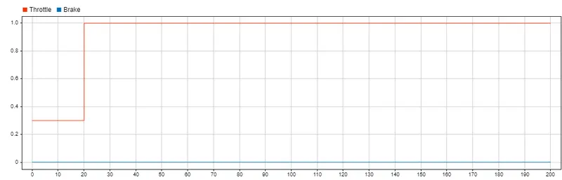
(i) Throttle and Brake input: In the first 20 secs the throttle input 0.3 given. After 20 secs full throttle is applied. however barke input

is kept at 0 for the whole simulation time.

Output:

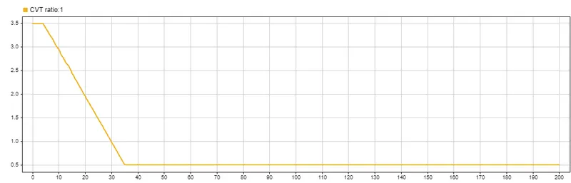
(i) CVT Ratio: After the simulation is completed, the plot of cvt ratio achieved as follows-

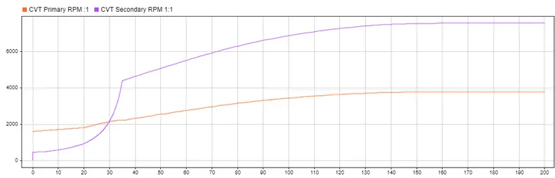
(ii) CVT RPM plot: The plot of primary and secondary rpm of cvt is shown as below-

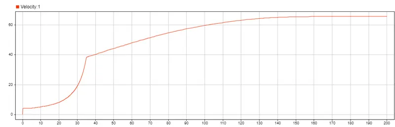
(iii) Velocity plot: The plot variation of velocity is fetched from the scope after the completion of simulation run. The top speed reaches around 64 kmph.

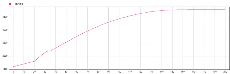
(iv) Engine RPM: The engine rpm plot is attached.

D. BAJA ATV Model with lookup table and dashboard:

A simulink model for baja atv with lookup table and dashboard is given below-

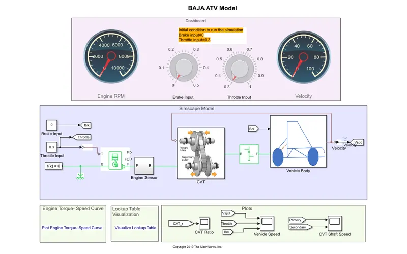
In this model we have added a dashboard to the close loop model as discussed above(model C). Here setup is quite same except the throttle and brake

inputs are going to be changed during run time. The initial conditions for the model are as follows-

Brake input = 0 ,

Throttle input =0.3

Lookup table data is same as the prevoius model.

Simulation Results :

The model is run for infinite time and inputs are varied during the simulation time by using the knobs in the dashboard. After running the model for quite a time,

simulation is stopped and plots were fetched from the scope.

Input:

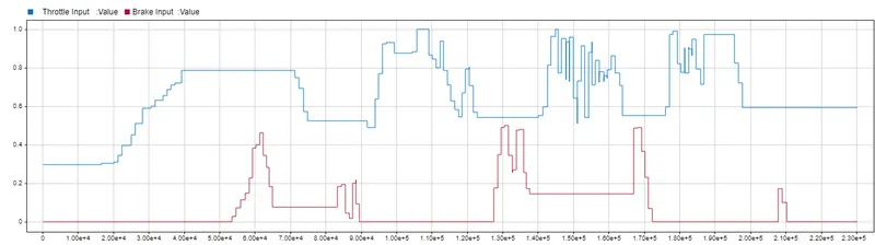
(i) Throttle and Brake : The throttle and brake inputs of the model are shown in the plot below-

Output:

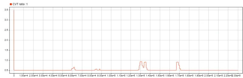
(i) CVT Ratio : The CVT ratio variation can be studied from the plot attached below. It stay at peak value of 3.5 during the start of simulation.

As throttle input is received, the cvt ratio decreases . During the instances when brake input is above 0.2, we can observe changes in cvt ratio.

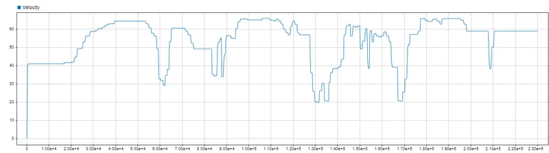
(ii) Velocity : The velocity curve fetched from the scope is as follows. We reach a top speed of 65 kmph (appx.).

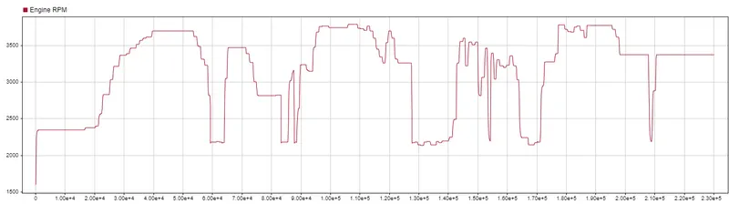
(iii) Engine RPM: The engine rpm variation plot is given below. The engine rpm varies as we vary throttle.

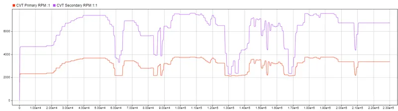
(iv) CVT RPM plot: The primary and secondary rpm plot of cvt is as follows-

Conclusion: The BAJA ATV's are really good vehicle for rough road conditions. These model give us basic knowledge knowledge of how atv's work and how CVT functons.

These simple models to get hands on experience of the baja vehicle and can give real insights in designing and manufacturing actual vehicles.

Referrences:

• Mathworks
• Models - https://www.mathworks.com/matlabcentral/fileexchange/70576-baja-all-terrain-vehicle-atv-model
• Matlab Documentation
• Baja SAE
• Youtube - Mathworks