State of charge estimation

Model Link

Battery Management Closed Loop Model Analysis.

There are two main blocks BMS and PLANT

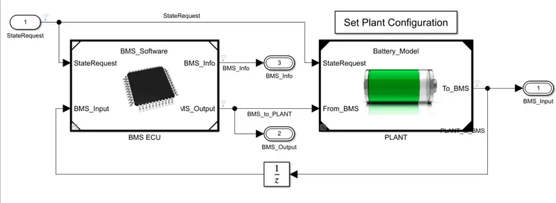
Plant:

Plant =( Battery pack + precharge circuit )which is connected to charger and load

the model here is a mathematical model in which the drive cycle is implemented as load just to study on the Battery MS

In the Charging circuit, there is a constant current source that charges the battery

1module= 6 series cells

Precharging circuit is used to avoid sparks and faults in the circuit due to sudden surge or rise in the current either while charging or discharging. and hence a resistor is connected first which reduces the transient time and makes sure that there is a gradual increase in the current.

BMS ECU

The battery management is implemented using a state model which in real life will be working as an IC which is fed with an algorithm in the form of a programming language or codes.

state machine takes in all the limits and indicates BMS state (B, C, d), and further, it commands contractors and gives signals.

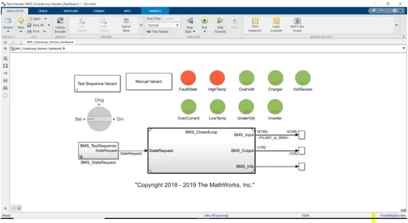
harness model.

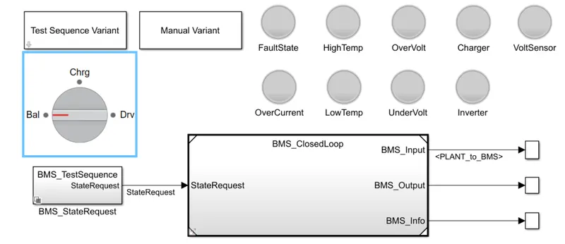
closed-loop with BMS

this dashboard gives information on the current situation, which will be indicated using the LED lights

there are three 3 BMS stand-by cases from the harness dashboard

1. Balancing
2. charging
3. discharging

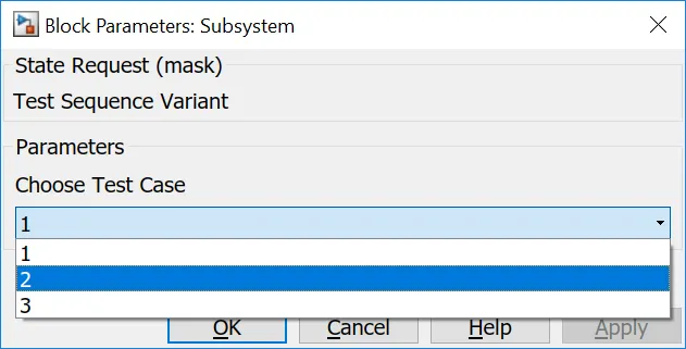
Test case 1: Driving-Balancing-Charging-Balancing

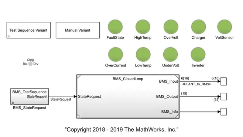
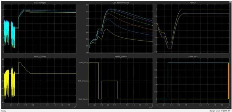
Finally, there is balancing after charging and discharging in the above test case, BMS is at the stand by the state that us neither charging nor discharging but it is working on cell balancing

Cell voltages: There is variation in voltages from 3.2 to 3.8 while the model was discharging and while charging the voltage is increased but when the BMS commands for cell balancing the voltages and SOC are set to 4.2 V and 100 percent respectively either by active or passive balancing

Cell_Temperatures: From the plot, we can observe there is 20 degrees variation in cells which is not a good situation and it should be taken into concern because the cell with higher temperature is affected and may end its life earlier than other cells thereby affecting the overall circuit and hence there needs to be proper thermal management.

SOC: The initial SOC was 80% which was then decreased to 50% and further while charging it completely charged. At constant current is charging there is a linear increase but when constant voltage there is a logarithmic increase.

BMS_State: from 0-0.2 there was discharging and 0.4- 0.9 there was charging and further it was stand by i.e cell balancing.

Peak_Current: Initially it was constant current charging(CCC) around 30A and later it was constant voltage charging(CVC), this can be observed in the plot when the current is constantly charging the voltage is almost linear increase and then vice-versa. CCC>CVC(TIME).

Test case 2: Drive-charge, High-temperature fault

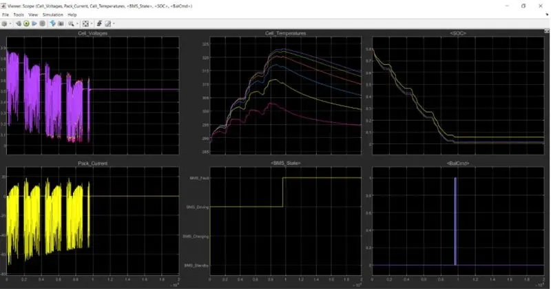
• The initial state of the voltage of all the cells is deflecting in the same manner and dropping slightly. It has 4 fluctuation zones and in between each of these fluctuating zone, they are stable for a while. The cells are initially at 80% SOC and then they're falling at different periods. to set their capability to recover. Other scopes indicate BMS state at each of the conditions.
• After 10,000 sec when the driving cycle is over, the fault condition occurs and so the SOC does not increase even for the charging phase.
• Cell temperature increases during driving, and since it is higher than recommended, BMS stops the battery from charging, so we can see a gradual decrease in temperature

Test case 3: Charging

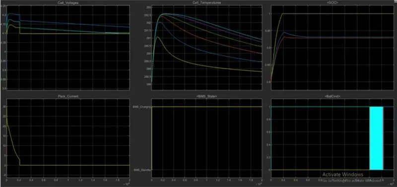
From the above graphs, all the cells are initiated at different voltages the where the 6 the one having the higher voltage of 4.2 V and the 1st one having near about 4.1 v and remaining falling under this range BMS on charging state throughout the simulation. So the voltage graph moves along in a straight line because the voltage supply continues. There is some deflection of voltage lines of different cells but that is a very less amount of change in voltage. At the end of the simulation, BMS tries to balance the voltage. The battery pack current is initiated with 20 A and then it falls to zero current till the end of the simulation. Then there is constant current because the battery is put in charge.

Graph 3 shows the temperature of the cells. The cells initiate at 287-degree Celcius temperature and then all the cells gradually see a decrease in temperature. The temperature difference at cell no 6 at its higher temperature will eventually cost much faster degradation of cell 6 compared to cell 1 leading to undesirable and unevenness in cell condition. therefore need an active thermal management system to keep thermal differences within a few degrees Celcius. The initial SOC of three different cells is at 80% as the. As the system is put on a charging state the SOC increases to 100% The other scopes indicate the BMS state at each of the balance command signals respectively. BMS on charging state and battery command passing signal between 0 to 1.

The SOC increases from 80 to 100% and then remains in standby mode. During charging SOC increases from 80 to 100%, temperature increases during charging and is reduced in the standby state of the BMS.

Coulomb counting

The Coulomb counting method is a method used to measure the discharging current of a battery. The method integrates the discharging current over time to estimate SOC. The Coulomb counting method is carried out to estimate the SOC at time t, which is estimated from the discharging current, I(t), and previously estimated SOC values, SOC(t-1). SOC is calculated by:

SOC(t)=SOC(t-1)+I(t)QnΔt">SOC(t)=SOC(t−1)+I(t)QnΔtSOC(t)=SOC(t-1)+I(t)QnΔt

There are several other factors affecting the accuracy of the Coulomb counting method including temperature, discharge current, battery history, and cycle life.

Limitations of coulomb counting: Coulomb Counting can be a very accurate technique, but it has its limitations:

• Leakage current within a cell does not go through the current sensor and is therefore not taken into account.

BMS implementation of coulomb counting for SOC estimation:

• The system does the estimation by the coulomb counting equation. The advantage of the coulomb counting method is its simplicity and low computational cost.
• Inside the BMS ECU block, we have the SOC estimation block.

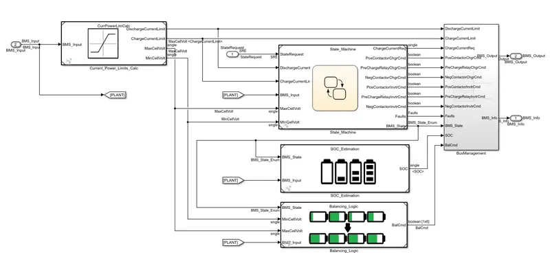
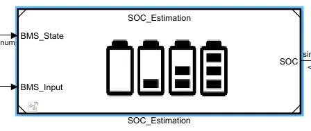
estimation three different formats.

the first is coulomb counting further UKF and EKF block which is Kalman filter indeed more accurate calculation then Coulomb counting.

Note; these effects can be observed in the above plot where the one which shows that the model is charged 100% is the coulomb counting method and the one that shows lesser than100% is the Kalman filter method, which indicates that the Kalman filter is more accurate in estimating SOC than coulomb counting method

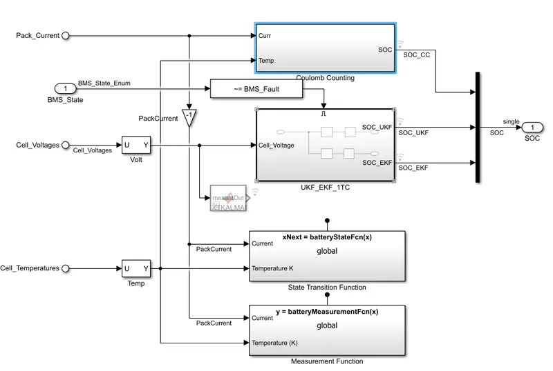
Coulomb counting is basically the integration of current over a period of time, which is done in discrete time integrator in z-domain.

• Within the coulomb counting, the SOC estimation is done.
• Temperature and current from the battery are given as inputs for coulomb counting.

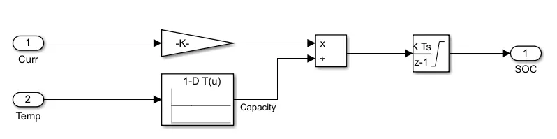
• The current signal is given to a gain block.
• These inputs are given for integration where the current will be integrated with respect to time.
• This output is given to another block where it is divided by capacity.
• This way the SOC is estimated