Week 7 State of charge estimation

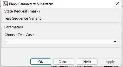
1. By observing the BMS Harness dashboard model results, the inferences are given below,

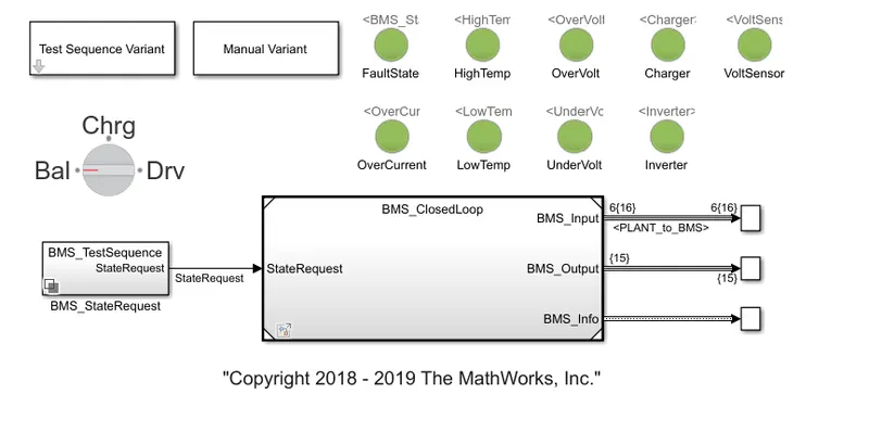
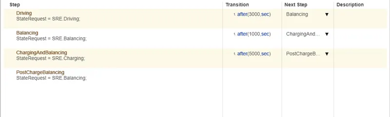
In Test case 1, the driving mode is from 0 to 3000 seconds, the balancing mode from 3000 to 4000 seconds and comes the charging mode and post balancing mode is from 4000 to 8000 seconds.

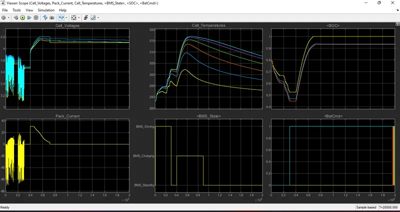
First Plot (Cell Voltage)

• The voltages of individual cells are shown and it fluctuates between 3.2 to 3.8v during the driving mode which is 0 to 3000 seconds.
• From 3000 seconds to 4000 seconds, there is a balanced voltage level of 4V which is obtained in the balance mode.
• From 4000 to 8000 seconds, there is a change in voltage level and increases to 4.2V, this is where the charging mode comes in.

Second Plot (Cell Current)

• From 0 to 3000 seconds, the current fluctuates from -60A and ends up to 0A during the driving mode.
• From 3000 to 4000 seconds, there is a balanced current level of 0A in the balance mode.
• From 4000 to 8000 seconds, there is a high spike to 30A during the charging mode.
• The current gradually decreases to 0A which occurs in the post balance mode.

Third Plot (Cell Temperature)

• The cell temperature increases and fluctuates during the driving mode and after the balancing mode, the temperature gradually decreases.

Fourth Plot ( BMS State )

• By observing the plot, the driving mode is between 0 to 3000 sec.
• The balancing mode occurs between 3000 to 4000 sec.
• The charging and post balancing mode occurs between 4000 to 8000 sec.

Fifth Plot ( SoC )

• During the driving mode, the SoC falls from 100% to 45%.
• During the balanced mode, the SOC is maintained at 45%.
• uring the charging mode, the SoC is increased from 45% to 100%.

Sixth Plot ( Balancing Command )

• This shows the balancing mode is from 3000 seconds.

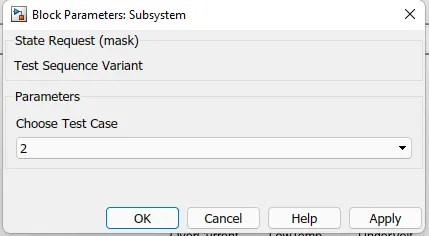
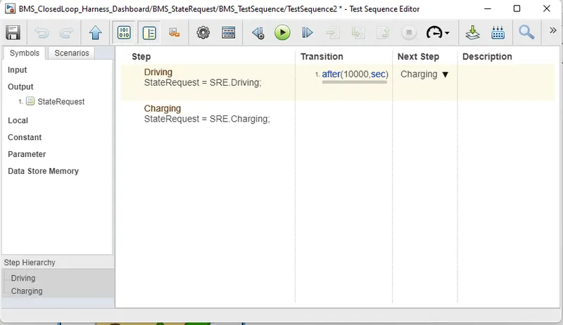
In Test case 2, the driving mode is from 0 to 10000 sec seconds and then comes the charging mode.

First Plot (Cell Voltage)

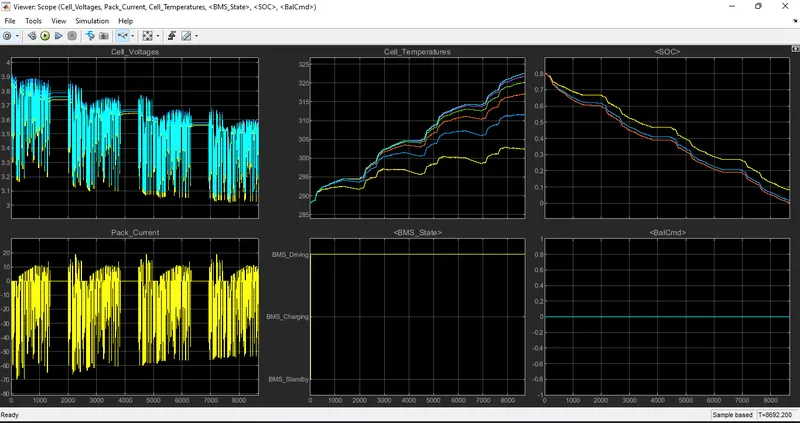
• The voltages of individual cells are shown and it fluctuates between 3.9 to 3.2v during the driving mode which is 0 to 8692 seconds.

Second Plot (Cell Current)

• From 0 to 8692 seconds, the current fluctuates between 0A and -60A during the driving mode.
• In between, there is a spike of 10A current.

Third Plot (Cell Temperature)

• The cell temperature increases during the driving mode from 0 to 8692 sec.

Fourth Plot ( BMS State )

• By observing the plot, the BMS graph shows all over from 0 to 8692 sec.

Fifth Plot ( SoC )

• During the driving mode, the SoC falls from 80% and gradually ends up 0%.
• Since there are no charging and balancing modes, the SoC keeps on decreasing.

Sixth Plot ( Balancing Command )

• This shows the balancing mode is from 0 to 8692 seconds.

Note: The plots shown are of 8692 seconds, although the driving mode is for 10000 seconds, the SoC gets to 0% in 8692 seconds. So, the vehicle runs for 8692 seconds only.

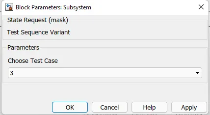
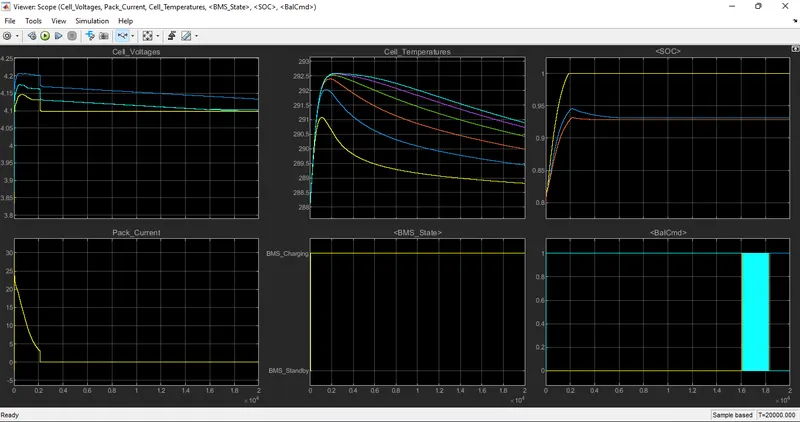
In Test case 3, the charging mode is from 0 to 20000 seconds and there are no driving and balancing modes.

First Plot (Cell Voltage)

• The voltages of individual cells are shown and it fluctuates for 20000 seconds and then it remains constant since charging is only taking place.

Second Plot (Cell Current)

• At a starting phase, there is a spike in pack current and it reaches 30A. It then reduces to 0A at 2000 seconds. From 2000 sec to 20000 sec, it remains constant at 0A.

Third Plot (Cell Temperature)

• The cell temperature increases during the charging mode from 0 to 1000 sec and gradually decreases from 1000 sec to 20000 sec.

Fourth Plot ( BMS State )

• By observing the plot, the BMS graph shows all over from 0 to 20000 sec.

Fifth Plot ( SoC )

• During the charging mode, the SoC increases from 80% and gradually ends up 100% in 2000 seconds.
• Since there are no driving and balancing modes, the SoC remains constant at 100%.

Sixth Plot ( Balancing Command )

• This shows the balancing mode is from 0 to 20000 seconds.

2. Coulomb counting is one of the methods to determine SoC (State of Charge). Soc is one of the important factors in battery systems. It is defined as the ratio of its current capacity to the total capacity.

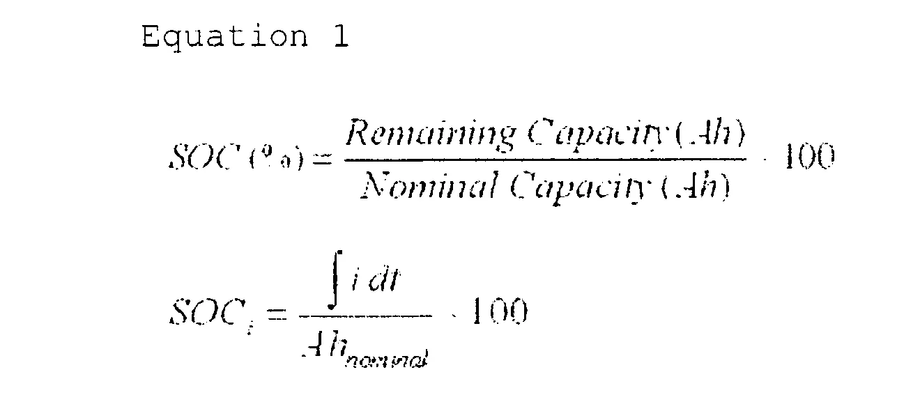
The total capacity represents the maximum amount of charge that can be stored in the battery. There are many ways to determine the SoC of a battery system,

• Direct Measurement
• Book Keeping estimation
• Adaptive systems

Direct Measurement

This method is done by considering the physical battery properties, such as the voltage and impedance of the battery.

Bookkeeping Estimation:

This method is done by observing the discharge current as of the input and calculates the Soc depending on the rate of discharging current over time.

Adaptive Systems:

This method is one of the advanced Soc determining systems as they can automatically adjust the Soc for different discharging patterns.

In the Book Keeping estimation method, there are two types followed namely,

• Coulomb Counting
• Modified Coulomb Counting

Coulomb Counting method:

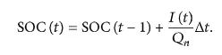
it measures the discharging current of a battery and integrates the discharge current over time to estimate Soc.

Coulomb Counting method is done to estimate the, which is estimated from the discharging current, and previously estimated SOC values, SOC is calculated by the following equation:

But several factors affect the accuracy of the Coulomb counting method including temperature, battery history, discharge current, and cycle life.

Modified Coulomb Counting method:

To improve the Coulomb counting method, a new technique called the modified Coulomb counting method is proposed. The modified Coulomb counting method uses the corrected current to improve the accuracy of estimation.

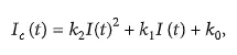
The corrected current is the function of discharging current. There is a quadratic relationship between the corrected current and discharging current of the battery. By the practice of experimental data, the corrected current is calculated by the following form:

where,

k0,k1,k2 are constant values obtained from the practice experimental data.

In the modified Coulomb counting method, SOC is calculated by the following equation:

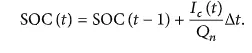
The experimental results show that the accuracy of the modified Coulomb counting method is superior to the conventional Coulomb counting method.

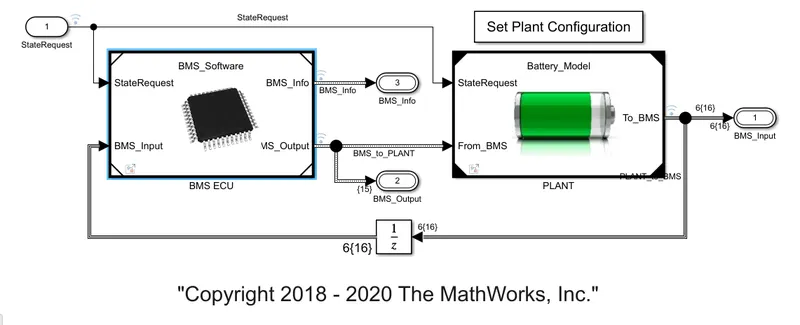
By observing the model, these are how a BMS implements coulomb counting for SOC estimation.

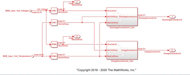
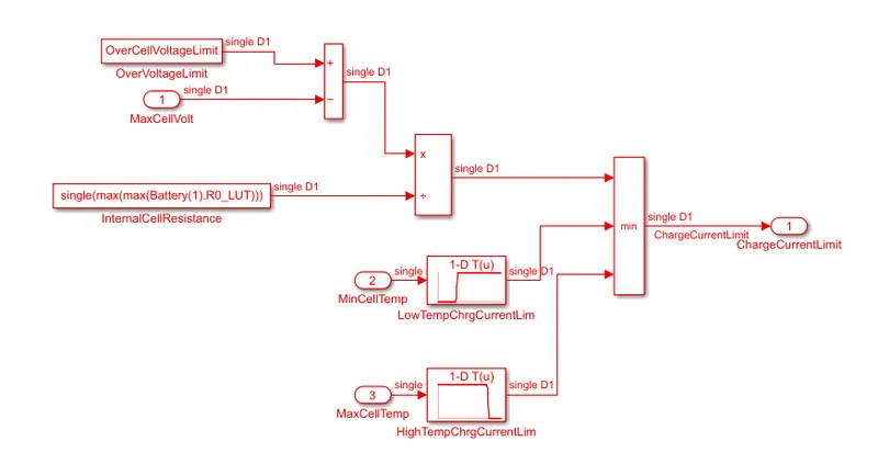
Click on the BMS ECU block, we can see the current power limit calc block. Inside that block, the cell voltage and cell temperature are used o decide maximum charging and discharging currents.

There are separate charge limit and discharging limit blocks. By clicking the discharge limit block, the result compares the minimum cell voltage and the threshold voltage and is divided by the internal cell resistance.

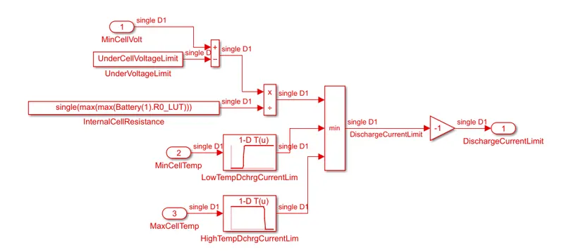
Using the lookup table, we can input the threshold-based temperature and modulate the allowable current delivery. It is used to maintain a low temperature during charging.

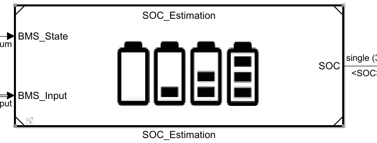
We can see the Coulomb counting used in this model by clicking onto the SoC estimation block ---> Coulomb counting block.

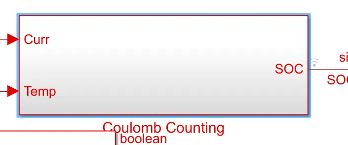
Here, the current and temperature is given as input. The current signal is fed into the gain block and the temperature signal goes to the current lookup table.

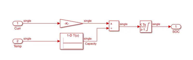
The temperature signal is the denominator and the multiplied current acts as the numerator and the two signals are fed to the integrator block and the SoC is estimated.

Advantages:

• Simplicity
• Low computational cost

Disadvantages:

• Current sensor error
• No feedback system for voltage computation.