Week-4 Challenge WOT Condition Part-2

1. The objective is to distinguish between the mapped and dynamic model of engine, motor, and generator,

Mapped Model	Dynamic Model
In this type of model, the data used for simulation is been fed as input in the form of a lookup table which would be configured and analysis can be done	In this type of model, the operation understands the behavior of the components and generates the output.
It is also known as Global Based Model	It is also known as Real-time Based Model
If the look-up table is of the required data, then the simulation can be done easily and the results can be accurate.	The results are dynamically operated by depending upon the situation of the operation and it delivers a detailed analysis of the simulation.
In engine or motor division, the engine/motor torque required is generated by mapping the input fed in the simulation without considering the engine/motor parameters.	Engine or Motor performance is analyzed with consideration of specifications and parameters specified for the vehicle in the simulation and the result are derived as real-time data.
The accuracy is not too high but it takes less time to simulate and gets the result.	The accuracy is high since it gets output from every subsystem and the data are real-time data but takes time for simulation.
The specifications of the engine, motor, and generator have top entered as data of the vehicle to be analyzed.	The specifications are also to be mentioned in the simulation it dynamically takes into consideration during the analysis of vehicles.
The only disadvantage is that more data has to be collected before the simulation	The only disadvantage is that the simulation cannot be done in custom specifications.

To change the model type in the Powertrain block Set,

• Firstly, we have to select the type of vehicle such as hybrid or fully Electric.
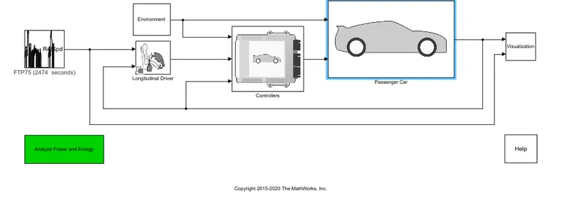
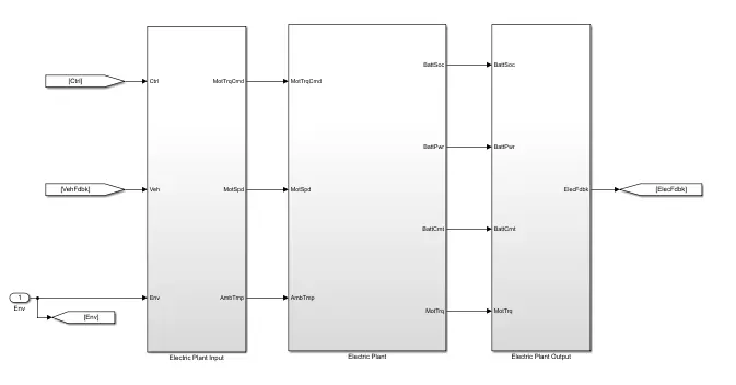
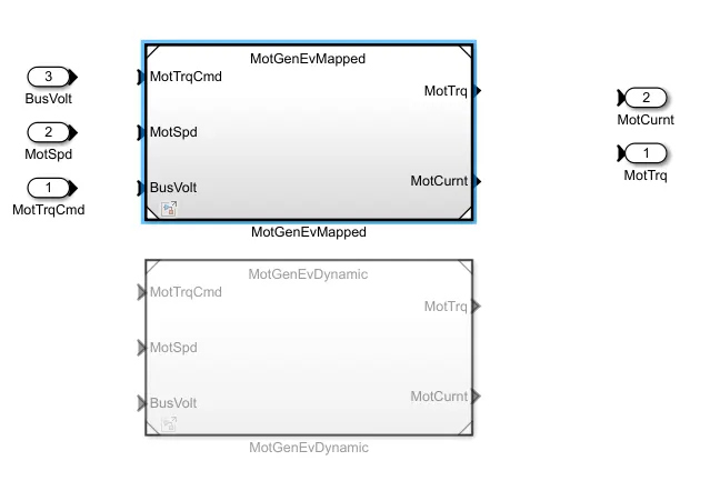
• In the EV Simulink model, go to Passenger car block > Electric Plant block > Ev Motor/Generator block.

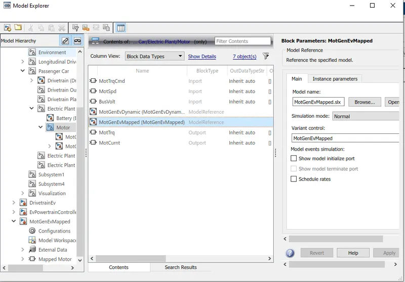
• Right, Click and select Explore.
• There has an option to switch between MotGenEV Mapped or MotGenEV Dynamic.

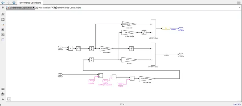
2. The objective is to analyze how does the model calculates miles per gallon and to find which are factors considered to model fuel flow.

• Miles per gallon term is the vehicle's fuel economy which represents the distance(miles) traveled by the vehicle for one gallon of petrol or diesel.
• The powertrain model has a block that calculates the miles per gallon.
• This considers the factors as input Vehicle Speed, Fuel Flow or Battery in case of Electric Vehicle.
• As the speed of the vehicle plays a vital role in the fuel economy of the vehicle, the distance traveled is determined by integrating the speed with time.
• By analyzing the Fuel Flow rate in gallon, this can be expressed in Litres by multiplying the resultant gallon by
  3.785 ( 264.172 gallon = 1000 litres)
• In the case of Electric vehicles, the fuel economy is calculated in terms of MPG and it can be expressed as KWh (Kilowatt Watt-hour) of electricity by multiplying the resultant gallon by 33.7 (1 gallon = 33.7 kWh).

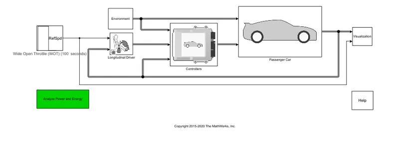
3. The objective is to run the HEV ReferenceApplication with WOT drive cycle and change the grade and wind velocity in the environment block.

• Firstly, we need to open the Hev reference model in Simulink and change the drive cycle input as WOT (Wide open Throttle).

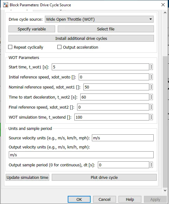
• In the block parameters, change the parameters to the desired values.

• Run the simulation and the observation from the results are listed below.

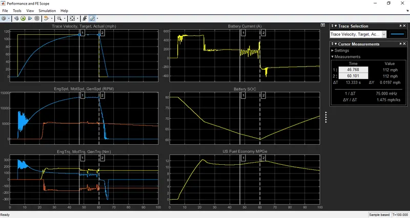
• Plot 1: Targeted Speed vs Actual Speed

In this plot, the vehicle can attain its maximum speed of 112 mph in around 47 seconds. The deceleration of the vehicle speed from 112 mph to 0 mph is done in 6.46 sec.

• Plot 2: Engine, Motor, and Generator Speed

In this plot, the speed curve of the motor is shown at various time intervals. The peak rpm of the motor is 13543 and for the motor and generator is 5726 rpm where the motor starts at 5 sec and the generator starts at 20 sec.

• Plot 3: Torque Characteristics

In this plot, the torque of the generator goes negative at 21 sec and it signifies that the battery is getting charged.

• Plot 4: Battery Current

In this plot, the motor is mainly used for the starting torque of the vehicle and it consumes a high current on the starting phase. A high current is drawn all over to 60 sec, and after 60 sec it drops to negative.

• Plot 5: Battery SoC

In this plot, initially, the battery charge is at 80% and the battery charge is drawn for vehicle acceleration, and at the end of the acceleration, the charge remains to be at 60%. At 25 sec, the battery starts charging

• Plot 6: Fuel Economy

In this plot, the fuel economy is calculated in US MPG and the maximum fuel economy attained is 12.04 MPG, and the minimum fuel economy obtained is 7.18 MPG.

To change the grade and wind parameters, go on to the Environmental block and give the desired values. In our case, I have given the grade and wind value as 10.

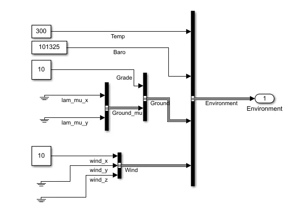
After running the simulation and observing the results, the conclusions are listed below.

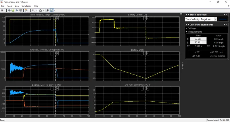
• Plot 1: Targeted Speed vs Actual Speed

In this plot, the vehicle can attain its maximum speed of 61.5 mph in around 58 seconds. The deceleration of the vehicle speed from 61.5 mph to 0 mph is done in 5.1 sec.

• Plot 2: Engine, Motor, and Generator Speed

In this plot, the speed curve of the motor is shown at various time intervals. The peak rpm of the motor is 7642 rpm and for the motor and generator is 5446 rpm where the motor starts at 5 sec and the generator starts at 20 sec.

• Plot 3: Torque Characteristics

In this plot, the torque of the generator goes negative at 21 sec and it signifies that the battery is getting charged.

• Plot 4: Battery Current

In this plot, the motor is mainly used for the starting torque of the vehicle and it consumes a high current on the starting phase. A high current is drawn all over to 60 sec, and after 60 sec it drops to negative.

• Plot 5: Battery SoC

In this plot, initially, the battery charge is at 80% and the battery charge is drawn for vehicle acceleration, and at the end of the acceleration, the charge remains to be at 60%. At 25 sec, the battery starts charging and at the end of the simulation, the charge remains at 71%.

• Plot 6: Fuel Economy

In this plot, the fuel economy is calculated in US MPG and the maximum fuel economy attained is 5.90 MPG, and the minimum fuel economy obtained is 4.3 MPG.

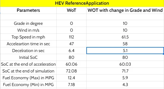
Thus, with lower grade and wind

• We can attain better acceleration in a short time
• We can attain better fuel Economy
• We can have better Soc

4. The objective is to run the HEV ReferenceApplication and EV ReferenceApplication with WOT drive cycle, change the grade and wind velocity in the environment block and compare the simulated results of hybrid and pure electric powertrains.

• Firstly, we need to open the HEV reference model in Simulink and change the drive cycle input as WOT (Wide open Throttle).

• In the block parameters, change the parameters to the desired values.

• Run the simulation and the observation from the results are listed below.

• Plot 1: Targeted Speed vs Actual Speed

In this plot, the vehicle can attain its maximum speed of 112 mph in around 47 seconds. The deceleration of the vehicle speed from 112 mph to 0 mph is done in 6.46 sec.

• Plot 2: Engine, Motor, and Generator Speed

In this plot, the speed curve of the motor is shown at various time intervals. The peak rpm of the motor is 13543 and for the motor and generator is 5726 rpm where the motor starts at 5 sec and the generator starts at 20 sec.

• Plot 3: Torque Characteristics

In this plot, the torque of the generator goes negative at 21 sec and it signifies that the battery is getting charged.

• Plot 4: Battery Current

In this plot, the motor is mainly used for the starting torque of the vehicle and it consumes a high current on the starting phase. A high current is drawn all over to 60 sec, and after 60 sec it drops to negative.

• Plot 5: Battery SoC

In this plot, initially, the battery charge is at 80% and the battery charge is drawn for vehicle acceleration, and at the end of the acceleration, the charge remains to be at 60%. At 25 sec, the battery starts charging

• Plot 6: Fuel Economy

In this plot, the fuel economy is calculated in US MPG and the maximum fuel economy attained is 12.04 MPG, and the minimum fuel economy obtained is 7.18 MPG.

To change the grade and wind parameters, go on to the Environmental block and give the desired values. In our case, I have given the grade and wind value as 10.

After running the simulation and observing the results, the conclusions are listed below.

• Plot 1: Targeted Speed vs Actual Speed

In this plot, the vehicle can attain its maximum speed of 61.5 mph in around 58 seconds. The deceleration of the vehicle speed from 61.5 mph to 0 mph is done in 5.1 sec.

• Plot 2: Engine, Motor, and Generator Speed

In this plot, the speed curve of the motor is shown at various time intervals. The peak rpm of the motor is 7642 rpm and for the motor and generator is 5446 rpm where the motor starts at 5 sec and the generator starts at 20 sec.

• Plot 3: Torque Characteristics

In this plot, the torque of the generator goes negative at 21 sec and it signifies that the battery is getting charged.

• Plot 4: Battery Current

In this plot, the motor is mainly used for the starting torque of the vehicle and it consumes a high current on the starting phase. A high current is drawn all over to 60 sec, and after 60 sec it drops to negative.

• Plot 5: Battery SoC

In this plot, initially, the battery charge is at 80% and the battery charge is drawn for vehicle acceleration, and at the end of the acceleration, the charge remains to be at 60%. At 25 sec, the battery starts charging and at the end of the simulation, the charge remains at 71%.

• Plot 6: Fuel Economy

In this plot, the fuel economy is calculated in US MPG and the maximum fuel economy attained is 5.90 MPG, and the minimum fuel economy obtained is 4.3 MPG.

• Firstly, we need to open the EV reference model in Simulink and change the drive cycle input as WOT (Wide open Throttle).

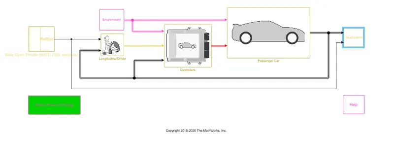
• In the block parameters, change the parameters to the desired values.

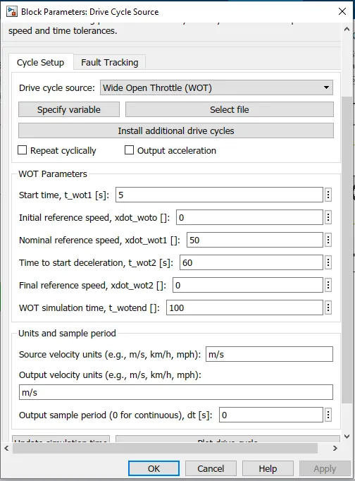
• Run the simulation and the observation from the results are listed below.

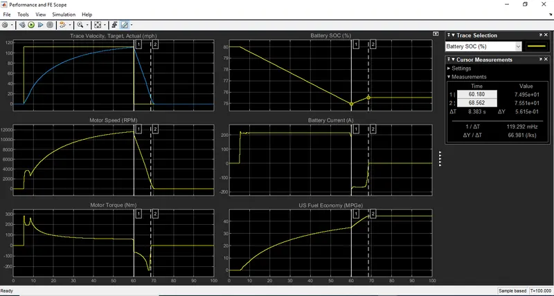
• Plot 1: Targeted Speed vs Actual Speed

In this plot, the vehicle can attain its maximum speed of 111.4 mph in around 59.8 seconds. The deceleration of the vehicle speed from 111.4 mph to 0 mph is done in 10. sec.

• Plot 2: Motor Speed

In this plot, the speed curve of the motor is shown at various time intervals. The peak rpm of the motor is 11620 where the motor starts at 5 sec.

• Plot 3: Torque Characteristics

In this plot, the torque of the motor goes negative at 60 - 66 sec and it signifies that the battery is getting charged.

• Plot 4: Battery Current

In this plot, the motor is mainly used for the starting torque of the vehicle and it consumes a high current on the starting phase. A high current is drawn all over to 60 sec, and after 60 sec it drops to negative.

• Plot 5: Battery SoC

In this plot, initially, the battery charge is at 80% and the battery charge is drawn for vehicle acceleration, and at the end of the acceleration, the charge remains to be at 74.95%. At 60 sec, the battery starts charging

• Plot 6: Fuel Economy

In this plot, the fuel economy is calculated in US MPG and the maximum fuel economy attained is 44.27 MPG, and the minimum fuel economy obtained is 34.86 MPG.

To change the grade and wind parameters, go on to the Environmental block and give the desired values. In our case, I have given the grade and wind value as 10.

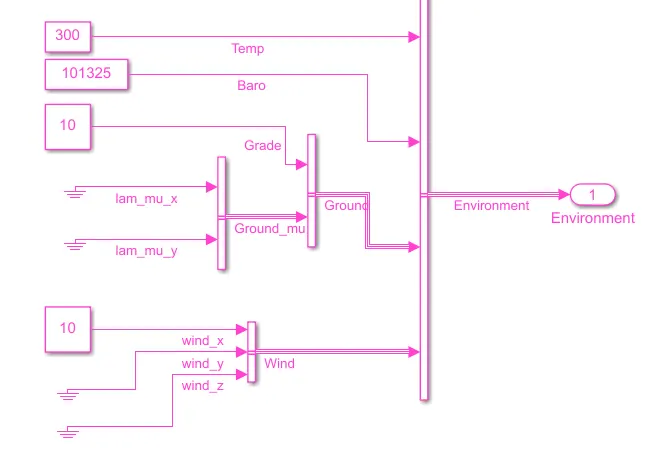
After running the simulation and observing the results, the conclusions are listed below.

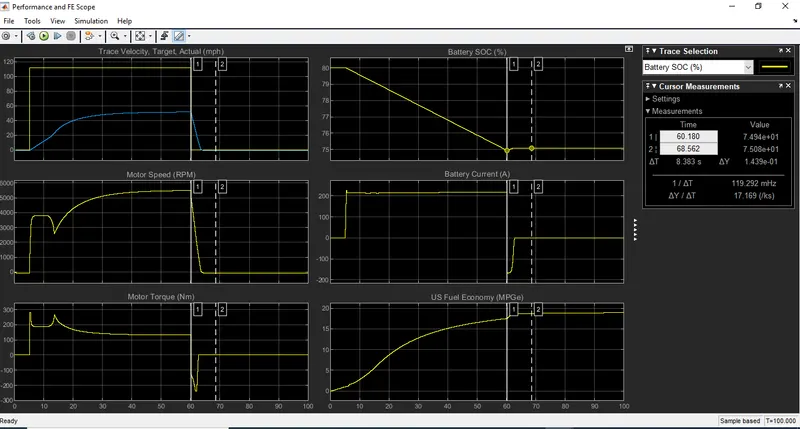
• Plot 1: Targeted Speed vs Actual Speed

In this plot, the vehicle can attain its maximum speed of 51.65 mph in around 59 seconds. The deceleration of the vehicle speed from 51.6 mph to 0 mph is done in 4.2 sec.

• Plot 2: Motor Speed

In this plot, the speed curve of the motor is shown at various time intervals. The peak rpm of the motor is 5497 where the motor starts at 5 sec.

• Plot 3: Torque Characteristics

In this plot, the torque of the motor goes negative at 60 - 64 sec and it signifies that the battery is getting charged.

• Plot 4: Battery Current

In this plot, the motor is mainly used for the starting torque of the vehicle and it consumes a high current on the starting phase. A high current is drawn all over to 60 sec, and after 60 sec it drops to negative.

• Plot 5: Battery SoC

In this plot, initially, the battery charge is at 80% and the battery charge is drawn for vehicle acceleration, and at the end of the acceleration, the charge remains to be at 74.97%. At 60 sec, the battery starts charging and the charge remains at 75.08% at the end of the simulation.

• Plot 6: Fuel Economy

In this plot, the fuel economy is calculated in US MPG and the maximum fuel economy attained is 18.70 MPG, and the minimum fuel economy obtained is 17.45 MPG.

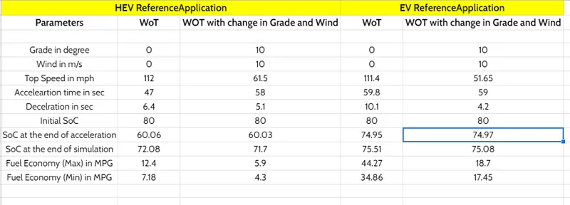
By comparing the results of HEV and Ev application simulation results, we can conclude that

• The Ev has the better SoC compared to Hevv at the end of the simulation.
• The Hev has better acceleration in a short time compared to Ev as it consists of a motor and engine.
• The Ev has better fuel economy compared to HEV even with the changes in parameters.