Week 7 State of charge estimation

State of Charge Estimation

1) Simulation of 3 test cases from harness dashboard:

Aim:

To simulate 3 test cases from harness dashboard for Design and Test Lithium-ion battery management algorithm and to make a detailed report.

Software used:

MATLAB/ Simulink

Procedure:

• Download the Design and test Lithium-Ion battery management algorithm.
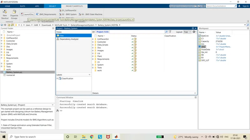
• Extract and open the plant model. And in the pop up window select open project and model.
• Launch the documentation from the top of the tab.

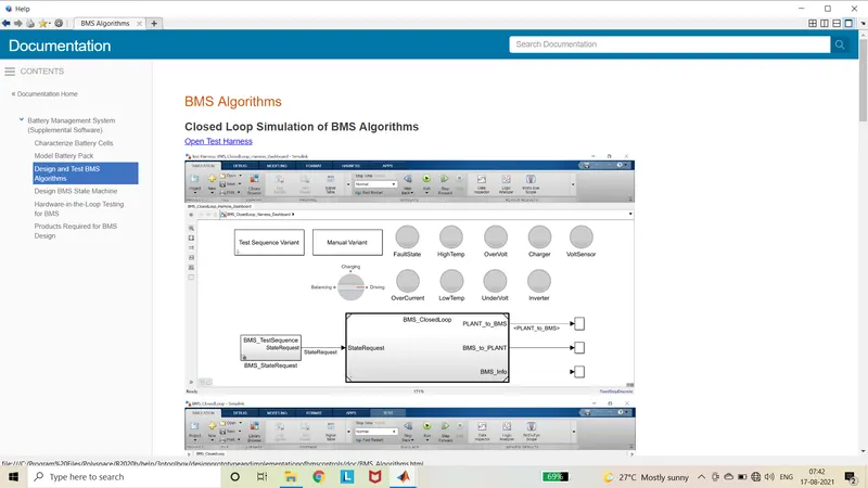
• Select Design and test, and click Open Harness model.

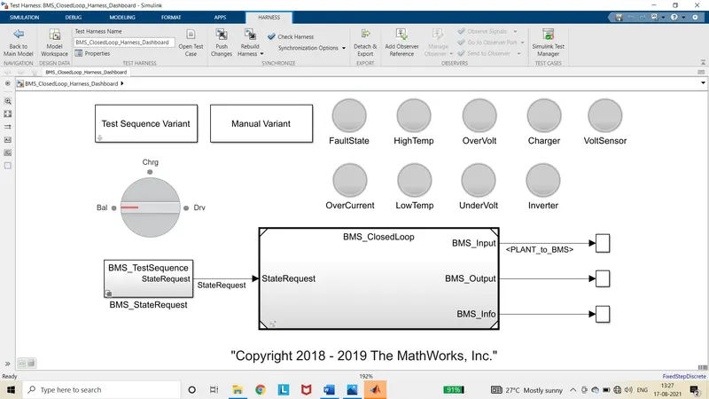
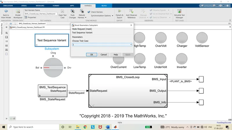
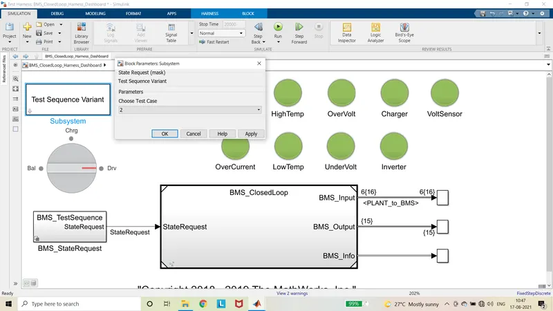
• Open test sequence variant and Choose the choice of test case we want as 1 or 2 or 3.

Test 1:

• First let us select 1.

• Then in the documentation window select Run simulation.

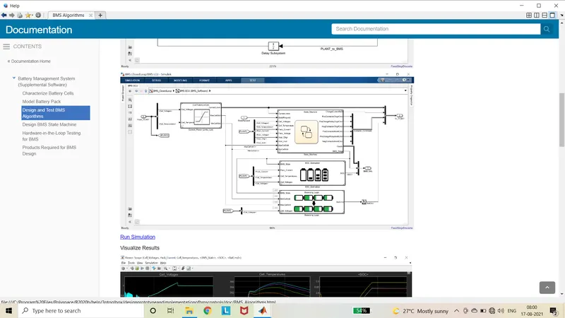
• The output scope opens and plot is visualized.
• For additional crosscheck, Open BMS_State request block and further open BMS_test sequence and test sequence 1.
• The steps for operation are given in test sequence editor.

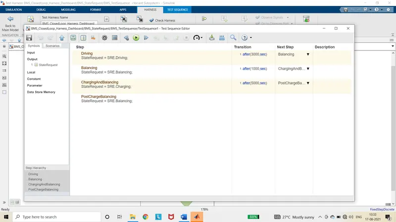
• The driving command state request is given for 3000 seconds, then it is followed by Balancing for 1000 seconds, then it undergoes charging and Balancing for 5000 seconds and then finally post charge balancing occurs for remaining simulation time.
• The total simulation time is 20000 seconds.
• The request commands are given to the BMS closed loop which contains BMS electronic control unit and Battery plant.
• These requests control the Stateflow chart.

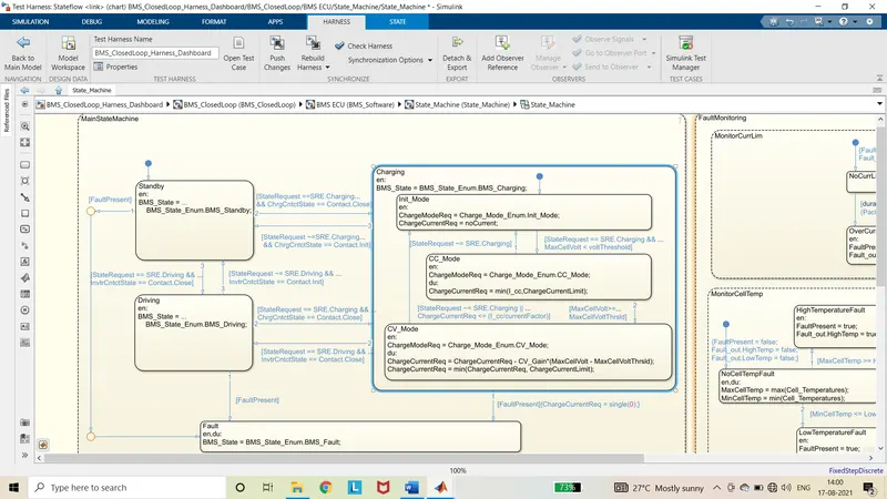
• This gives commands to battery plant model and controls the actions.

Output:

Summary:

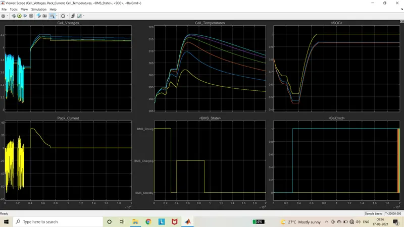
From the above plot, it is observed that, the pack voltage reduces while driving (discharging) till 3000 seconds. During this time the current is more negative this implies that negative current is for discharging ang and positive for charging. BMS state indicates the system is driving for 3000 seconds and the state of charge decreases from 80% to 45%.

For the 3000 – 4000 seconds the system is in standby mode, the voltage, current and SoC are remains constant. The temperature of cell 6 is maintained constant and other cell temperatures are reduced. The cell 6 balancing takes place during this time.

For 4000 - 9000 seconds the system is in charging mode as indicated by the BMS state. During this time CCCV charging occurs. For first 500 seconds, the constant current charging takes place. The constant current of 30A is given for charging. During that time pack voltage increases near to 4.2V then the constant voltage charging takes place. This takes place for long duration of time. i.e) for 4500 seconds. During this duration of time the current is reduced gradually. When the current is reduced to zero. Then the voltage is slightly reduced and maintained constant. The cell temperature is increased during the constant current mode of charging and reduces during charging and standby mode. The State of charge is increased to 100% as per coulomb counting method. But Kalman’s method of calculation of SOC is around 93%.

For 9000 to 20000 the system is in standby mode, the current and soc remains constant. The cell balance is done by constant impulse at the end of the cycle from 19500 to 20000 seconds. The voltage of the cells is tried to make more or less equal.

Test 2:

• Open test sequence variant and choose the choice of test case 2.
• Run the simulation and visualize the output.
• For additional crosscheck, Open BMS_State request block and further open BMS_test sequence and test sequence 2.

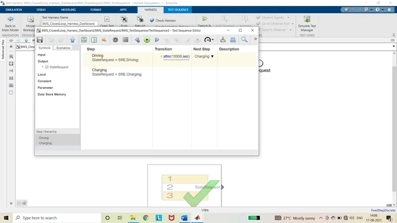
• The requests are driving for 10000 seconds and then charging for remaining time.

Output:

Summary:

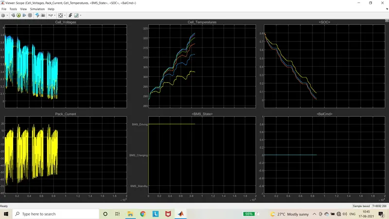
From the above plot it is observed that the system is in driving state the battery gets discharged. The voltage gets reduced and the current is in negative direction which implies that the discharge current is negative. The cell temperature is increased rapidly during discharge and state of charge is decreases rapidly. The BMS state implies the driving mode. The system stops once the state of charge becomes 0% at 8692 seconds. But the state flow condition is the system has to drive for 10000 seconds and after that it has to charge for 10000 seconds. But because of state of charge becomes 0 the system stops. The cell balancing remains zero because there is no charging.

Test 3:

• Open test sequence variant and choose the choice of test case 3.
• Run the simulation and visualize the output.
• For additional crosscheck, Open BMS_State request block and further open BMS_test sequence and test sequence 3.

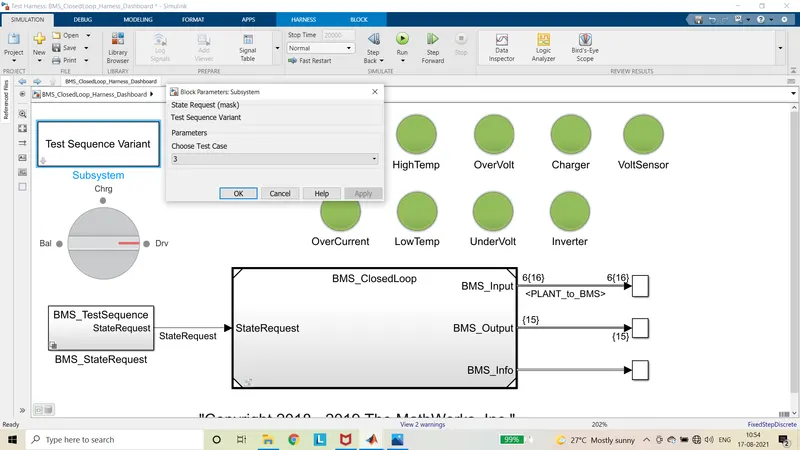
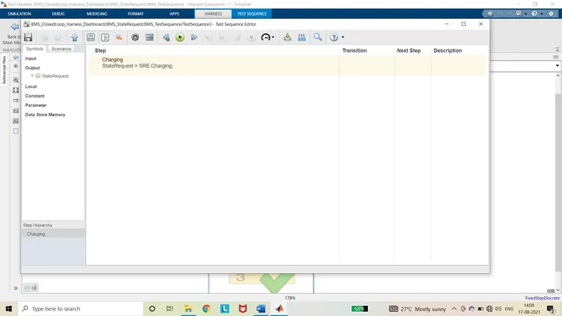
• The only request operation is charging.

Output:

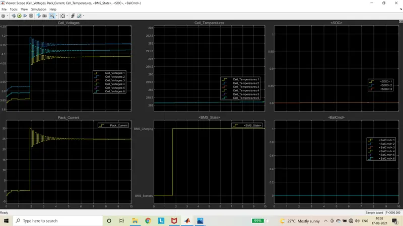
Zoomed In view:

Summary:

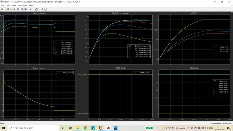
From the above plot, it is observed that only charging occurs in this test case. The charging type is CCCV (constant current constant voltage). Initially the charging mode is constant current charging, this is visualized in the zoomed in view of the plot. The impulse current of 30A is given and is gradually reduced and maintained constant of around 25A for small period of time till the voltage reaches the preset value. Once the preset value is reached, the constant voltage charging occurs. The voltage is constant and the current is gradually reduced to minimum value. Once the current is reduced to zero there is some slight reduction in the voltage of the cell. The temperature of the cell is increased during the constant current charging and starts to decease after that. But the cell number 5 and 6 temperatures remain constant. This may be because of the arrangement of cell in the pack. The SoC is 100% around 2000 seconds for Coulomb counting method. And for Kalman’s method of calculation the SoC is around 94% and 93%.

2) Coulomb Counting and SOC estimation:

Aim:

To study about Coulomb counting and to explain how BMS implements coulomb counting for SOC estimation.

Coulomb Counting:

Coulomb counting method uses the current through the battery whether it is discharge current or charge current and it is integrated over the time to estimate the SOC of the battery at an instant. This method is estimated current, total capacity and the previous SOC value. The temperature also affects the SOC estimation.

`SOC(t) = SOC (t-1) *int( I(t)*(dT))/Q`

dT = change in time

Q = total capacity.

Since integration of current over time is the charge and this method counts the charge. The unit of charge is Coulomb. Hence it is called as Coulomb counting method.

`I = (dq)/dt`

`intI.dT=q`

Procedures for SOC estimation using Coulomb counting:

• The coulomb counting takes place in the SOC estimation subsystem of BMS Electronic control unit subsystem.

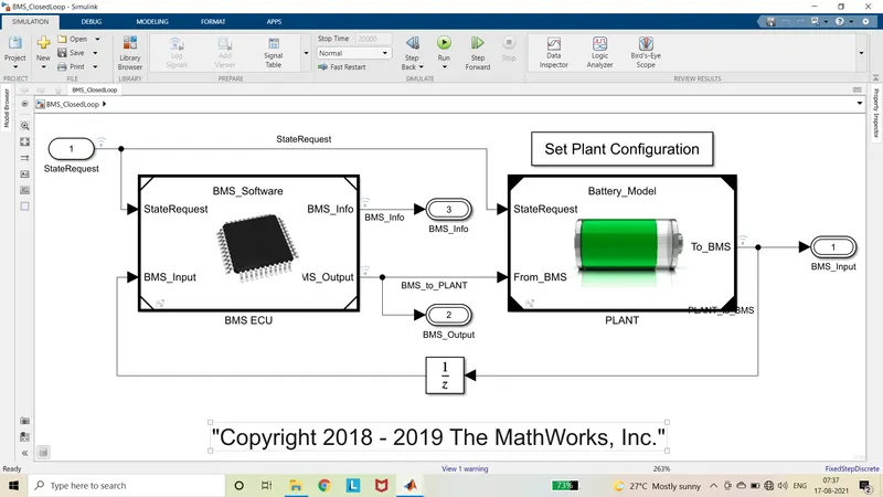
• The output of the battery plant are feed back to the BMS ECU.
• This is given as one of the inputs to the SOC estimation subsystem.
• It provides the pack current and cell temperature required for the coulomb counting method.

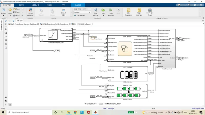
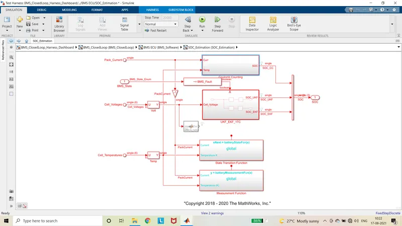
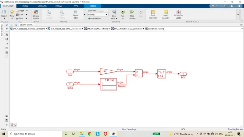
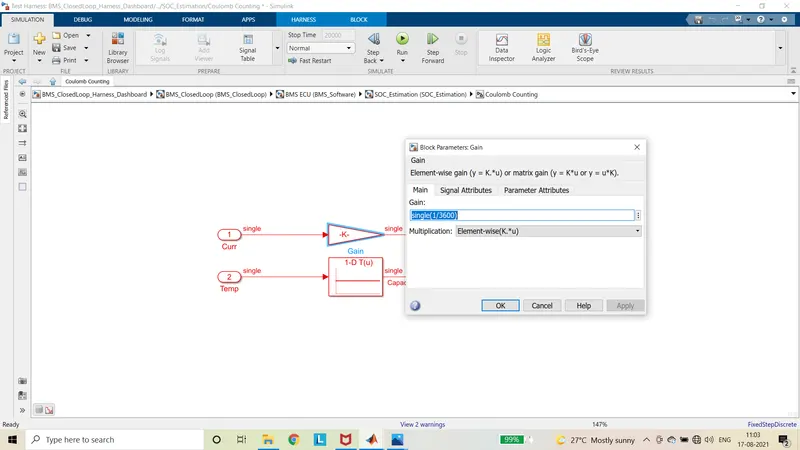
• The Input pack current is multiplied with the gain value of (1/3600) which is used to convert the current in A to Ah and is divided with capacity of battery.
• The capacity of battery is given with respect to temperature using the Lookup table block.
• This is then integrated over the time to give depth of discharge value.
• This is subtracted from the Initial SOC to get the instantaneous State of Charge.

Summary:

From the above mentioned equation, the blocks are made according to that to estimate the State of charge. It is easy to calculate but it is associated with some error. The estimation error is about 11.4%. The SOC estimation using Kalman’s is about 2.3%.

Drive Link:

https://drive.google.com/drive/folders/10okcWoFvWdtPQA12eLKKNQEklKCkvZOM?usp=sharing