Week 7 - Simulation of a 1D Supersonic nozzle flow simulation using Macormack Method
ASSIGNMENT
THEORY :
Consider a general flow field represented by the streamlines as shown in the figure . Also consider a closed volume defined by V , with a surface S. This surface bounds the flow. The CV can be seen in two ways
- Fixed in space and the fluid moving through it
- Control volume moving with the fluid.
In the first case the CV is fixed and fluid flows through it, so the fluid particle inside the CV keeps chanhing . In the second case, it is the same fluid particle that that is enclosed within the CV and this CV flows with the fluid. To these to CVs , we apply the conservation principles- mass , momentum and energy .
The equation obtained either in the integral or differential form for the CV fixed in space is the conservative form of the equation and the equations obtained from the CV moving with the fluid is the non conservative forms of the differential equation.
non conservative form : `(Drho)/(Dt)+rho grad.V=0`
Conservative form : `(Drho)/(Dt)+ grad(rho.V)=0`
PROBLEM STATEMENT AND EQUATIONS USED:
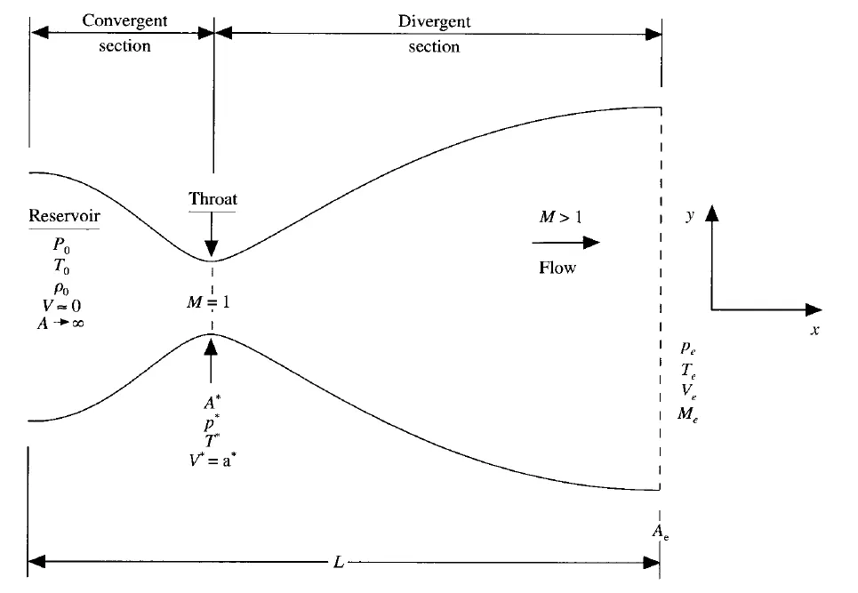
Fig 1
The flow considered here is a steady isentropic flow through a convergent divergent nozzle. The flow at the nozzle inlet comes from the reservoir where the pressure and Temperature are Po , To respectively. The cross sectional area at the reservoir is large and therefore the area is infinite so , the velocity `Vo` is 0. The flow expands isentropically to supersonic speeds at the nozzle exit and the values are given in the figure above. The flow is subsonic at the convergent section , sonic at the throat and supersonic at the divergent section.
ASSUMPTIONS :Here we make an assumption that the flow properties vary only in the x direction because of which, its a Quasi 1D flow.
The governing equations for the quasi 1D flow are:
Continuity : `p1 A1 V1=p2 A2 V2`
Momentum : `rho1.A1 + rho1.A1.V1^2 +int_(A_1)^(A_2) rho dA =rho2.A2+rho2.A2.V2^2`
Energy : `h1+(V1^2)/2 = h2+(V2^2)/2`
In addition we also have the equation of state given by :
`P=pRT`
CFD solution :
In this project , we solve the 1D isentropic convergent divergent nozzle problem using the Maccormack's discretization technique. This technique is a two step technique, which involves a predictor step and a corrector step. The steps for solving this is give below :
1. 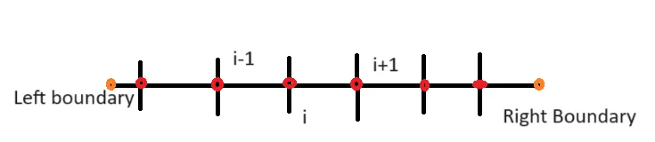
consider this 1D mesh. Assume it to be equidistant. Here we are looking for a time marching solution. In this we use explicit time marching.
2. It begins by calulating the predictor step using the initial conditions. Suppose 'f' is the quantity we are interested in , the first step is to get the predictor step given by :
`(delf)/(delt_p)`
3. Once this is calculated ( in the problem, we do this for mass, momentum and energy), we do an intermediate solution update.
`f^(*) =f_i + ((delf)/(delt_p)*dt)`
here fi is the initial condition.
4. One thing to be noted is that for the predictor step, a forward differencing is used.
5. Now with the predictor values, we use to find the corrector values or perform the corrected step , which is
`(delf)/(delt_c)`.
6. Once we have the corrector step, we perform an average of the predictor and corrector values
`(delf)/(delt_(avg))=((delf)/(delt_(c))+(delf)/(delt_(p)))*0.5`
7. Once the average value is obtained, we find the final value for the next time step by performing step 3. We add the average value to the initial value.
`f_(f) =f_i + ((delf)/(delt_(avg))*dt)`
CONSERVATIVE AND NON CONSERVATIVE FORM
The project here aims to solve the convergent divergent problem both using the conservative and the non conservative form.
NON CONSERVATIVE FORM
The equations used in the non conservative form are :
Continuity Equation :`(delrho' )/(delt)= -rho' (delV')/(delx')-rho'V'(del lnA)/(delx')-V'(delrho')/(delx')`
Momentum Equation : `(delV')/(delt')=-V'(delV')/(delx')-1/gamma((delT')/(delx')+(T')/(rho') (delrho')/(delx'))`
Energy Equation :
Continuity Equation : `(delT')/(delt')=-V'(delT')/(delx')-(gamma-1)T'((delv')/(delx')+V'(dellnA')/(delx'))`
One thing to be noted is that the the values with the apostroph are dimensionless variables. They are represented as follows :
`T'=T/T_o` `rho'=rho/rho_o` `x'=x/L`
T_o , rho_o are the reservoir temperature and density and L is the total length of the nozzle
`a_o=sqrt(gamma R T` where a_o is the speed of sound
`V'=V/a_o`
`A**=A/A_o` where A_o is the throat area
`t'=t/(L/a_o)` where L/a_o is the equivalent of time
CONSERVATIVE FORM
When it comes to conservative form , though the concept is same, the approch is a little different. We have the equations as follows:
Continuity : `(delrho'A')/(delt')'+(delrho'A'V')/(delx')=0`
momentum : `(delrho'A'V)/(delt')+(delrho'A'V'^2+(1/gamma*rhoA))/(delx) = 1/gamma (delA')/(delx')rho`
energy equation : `(delrho((e^'/(gamma-1)+V'^2gamma/2))A')/(delt')+ (delrho((e^'/(gamma-1)+V'^2gamma/2))A'V'+rho'A'V')/(delx')=0`
The above equations are the non dimensional conservative forms of the mass momentum and the energy equations. The equation can be expressred in a different form similar to
`(delU)/(delt)+(delF)/(delx)+(delG)/(dely)+(delH)/(delz)=J`
here F G and H are called the flux vectors, U is the solution vector and J is the source term. In this example we define the solution U, Flux F and Source J as follows
`U1=rho'A'`
`U2=rho'A'V'`
`U3=rho(e/(gamma-1)+1/gamma(V'^2)/2)A`
`F1=rho'A'V'`
`F2=rho'A'V'^2 +(1/gamma)rho'A'`
`F3=rho'((e')/(gamma-1)+(y/2)*V'^2)A'V' +rho'A'V'`
`J2=1/gammarho'(delA')/(delx')`
With U1 U2 U3 F1 F2 J2 respectively, we represent the continuity, moemntum and energy equations as follows
`(delU1)/(delt')=-(delF1)/(delx')`
`(delU2)/(delt')=-(delF2)/(delx')+J2`
`(delU3)/(delt')=-(delF3)/(delx')`
Important thing to note is that in the conservation form of the equations, the dependent variables are not the primitive variables.We get numbers directly for U1 U2 and U3. That is why they are called the solution vectors.
You can calculate the primitive variables from U1 U2 and U3 respectively, the formulas are given below :
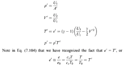
( taken from John D Andersson text)
Due to instabilities occured , its best to construct F1 F2 F3 and J2 from U1 U2 and U3
`F1=F1(U1 ,U2, U3)`
`F2=F2(U1 ,U2, U3)`
`F3=F3(U1 ,U2, U3)`
`J2=J2(U1 ,U2, U3)`
the formulas are given below :
`F1=U2`
`F2=((U2)^2/(U1))+(gamma-1)/gamma(U3-gamma/2 (U2^2)/(U1))`
`F3=gamma(U2 U3)/(U1)-gamma((gamma-1)/2)(U2^3)/(U1^2)`
similarly
`J2=(gamma-1)/gamma (U3-gamma/2(U2^2)/(U1^1))(dellnA')/(delx')`
BOUNDARY CONDITIONS
Coming to the boundary conditions,
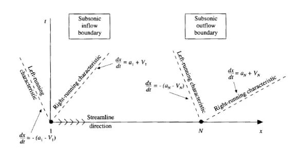
(figure taken from John D Andersson text)
The we need to understand the characterstics of a hyperbolic PDE. Since its a time marching problem , the PDES are hyperbolic, so there will be two characteristic curves. At grid point 1, the the local flow velocity is subsonic so the left running characterstics is going out of the domain against the mach wave . Due to the nature of flow and the direction of streamlines , values of 2 dependent variables must be specified at the inlet and one to float, and at the outlet, all variables must be allowed to float.
The conditions for conservative and non conservative forms are given below :
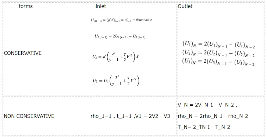
The initial conditions are given as a function of x for density and temperature for both the conservative and non conservative cases( as per the text book). It is also implemented in the code.
CODE , RESULTS AND DISCUSSION
The main code is give below
clear all
close all
clc


x=linspace(0,3,31); % number of nodal points

dx= x(2)-x(1)
C=0.5
nt=1400;
gamma=1.4;

choice=input('enter the choice 1 or 2');

if choice==1
    tic
    [pre,Mach,m,rho, V, T ,rho_t , V_t, T_t, P_t, M_t, m_t]=non_conservation(x, dx,C ,nt, gamma)
    time_elapsed_NC=toc;
else
    tic
    [pre,Mach,m,rho, V, T ,rho_t , V_t, T_t, P_t, M_t, m_t]=conservation(x, dx,C ,nt, gamma)
    time_elapsed_C=toc;
end


analytical_massflow=0.579*ones(1400,1);
analytical_mach=1*ones(1400,1);
analytical_temp=0.833*ones(1400,1);
analytical_density =0.634*ones(1400,1);
analytical_pressure =0.528*ones(1400,1);


figure(2)
subplot(5,1,1)                          %mass flow
plot(1:1400, m_t, 'g','linewidth',1.5)
hold on
plot(1:1400, analytical_massflow, 'm','linewidth',1.5)
xlabel('timestep variation')
ylabel('mass flow rate at the throat')
legend({'calculated mass flow at the throat','analytical mass flow'});
grid on
title(' Comparison of variables  at the throat')

subplot(5,1,2)               %mach number
plot(1:1400, M_t, 'g','linewidth',1.5)
hold on
plot(1:1400, analytical_mach, 'm','linewidth',1.5)
xlabel('timestep variation')
ylabel('Mach number at the throat')
legend({'calculated mach number  at the throat','analytical mach number'})
grid on;

subplot(5,1,3)              %temperature
plot(1:1400, T_t, 'g','linewidth',1.5)
hold on
plot(1:1400, analytical_temp, 'm','linewidth',1.5)
xlabel('timestep variation')
ylabel('Temperature at the throat')
legend({'calculated temperature at the throat','analytical temperature'})
grid on;


subplot(5,1,4)            %density
plot(1:1400, rho_t, 'g','linewidth',1.5)
hold on
plot(1:1400, analytical_density, 'm','linewidth',1.5)
xlabel('timestep variation')
ylabel('density at the throat')
legend({'calculated density at the throat','analytical pressure'})
grid on;

subplot(5,1,5)            %pressure
plot(1:1400, P_t, 'g','linewidth',1.5)
hold on
plot(1:1400, analytical_pressure, 'm','linewidth',1.5)
xlabel('timestep variation')
ylabel('pressure at the throat')
legend({'calculated pressure at the throat','analytical pressure'})
grid on;

figure(3)
subplot(5,1,1)                          % pressure along the length of the nozzle
plot(x, pre, 'g','linewidth',1.5)
xlabel('distance (x) along the nozzle')
ylabel('pressure variation')
grid on
%title(' Comparison of variables  along the length of the nozzle')

subplot(5,1,2)                          % temp along the length of the nozzle
plot(x, T, 'g','linewidth',1.5)
xlabel('distance (x) along the nozzle')
ylabel('temperature variation')
grid on
%title(' Comparison of variables  along the length of the nozzle')

subplot(5,1,3)                          % velocity along the length of the nozzle
plot(x, V, 'g','linewidth',1.5)
xlabel('distance (x) along the nozzle')
ylabel('velocity variation')
grid on
%title(' Comparison of variables  along the length of the nozzle')

subplot(5,1,4)                          % mach along the length of the nozzle
plot(x, Mach, 'g','linewidth',1.5)
xlabel('distance (x) along the nozzle')
ylabel('mach variation')
grid on
%title(' Comparison of variables  along the length of the nozzle')

subplot(5,1,5)                          % mach along the length of the nozzle
plot(x, rho, 'g','linewidth',1.5)
xlabel('distance (x) along the nozzle')
ylabel('density variation')
grid on
%title(' Comparison of variables  along the length of the nozzle')
Code for non-conservation form
function[pre,Mach,m,rho, V, T ,rho_t , V_t, T_t, P_t, M_t, m_t ]=non_conservation(x, dx,C ,nt, gamma)

    clear all
    close all
    clc

    n=31;
    x=linspace(0,3,n); % number of nodal points

    dx= x(3)-x(2)
    C=0.5
    nt=1400;
    gamma=1.4;
    throat=(n+1)/2


    %initial conditions

    A  =  1 +( 2.2*(x -1.5).^2) ;                    % area where x varies from 0 to 3
    rho =  1-(0.3146*x)       ;                      % variation of density WRT x
    T =  1-(0.2314*x)          ;                      %temperature variation
    V = (0.1+(1.09*x)).*T.^0.5  ;                     %velocity variation
    drhodt=0;


    for it=1:nt


        %calulating the time step
        %dt_1=(C.*dx./(sqrt(T)+V))
        dt= min(C.*dx./(sqrt(T)+V))  ;

        %storing the old values
        rho_old = rho;
        T_old = T;
        V_old = V;

        %predictor step
        for i=2:n-1

            d_rho_dx = (rho(i+1) - rho(i)) / dx;
            d_v_dx_p = (V(i+1) - V(i)) / dx;
            d_T_dx_p = (T(i+1) - T(i)) / dx;
            d_logA_dx = (log(A(i+1)) - log(A(i))) / dx;

            % Continuity equation
            d_rho_dt_p(i) = -(rho(i) * d_v_dx_p) - (rho(i) * V(i) * d_logA_dx) - (V(i) * d_rho_dx);

            % Momentum equation
            d_V_dt_p(i) = -V(i) * d_v_dx_p - (1/gamma) * (d_T_dx_p + (T(i) / rho(i)) * d_rho_dx);

            % Energy equation

            d_T_dt_p(i) = -V(i) * d_T_dx_p - (gamma-1) * T(i) * (d_v_dx_p + (V(i) * d_logA_dx));


            %updating the solution of the predictor step

            rho(i)=  rho(i)+ ( d_rho_dt_p(i)*  dt);
            V(i)=    V(i)+  ( d_V_dt_p(i)*  dt);
            T(i)=    T(i)+ ( d_T_dt_p(i)* dt);

        end

        %corrector step
        for i=2:n-1

            d_rho_dx= ( rho(i)-rho(i-1)) / dx;
            d_v_dx= ( V(i)-V(i-1)) / dx;
            d_T_dx= ( T(i)-T(i-1)) / dx;
            d_logA_dx= ( log(A(i))-log(A(i-1) ) )/ dx;

            % continuity equation

            d_rho_dt_c(i)=-(rho(i)*d_v_dx)- (rho(i)*V(i)* d_logA_dx)- (V(i)* d_rho_dx);
            %drhodt_p(j)=-rho(j)*dvdx_p-rho(j)*V(j)*dlogA_dx_p-V(j)*drhodx_p;

            %momentum equation

            d_V_dt_c(i)=(-V(i)*d_v_dx)-  ((1/gamma* (d_T_dx) )+ (T(i)/rho(i)* d_rho_dx) );
            %dvdt_p(j)=-V(j)*dvdx_p-(1/gamma)*(dtdx_p+(T(j)/rho(j))*drhodx_p);

            %energy equation

            d_T_dt_c(i)=( -V(i)*d_T_dx )- ((gamma-1)*  T(i)*  (d_v_dx+(V(i)* d_logA_dx)));
            %dtdt_p(j)=-V(j)*dtdx_p-(gamma-1)*T(j)*(dvdx_p+V(j)*dlogA_dx_p);

        end

         %computing the average of predictor and corrector

         drhodt= 0.5*(d_rho_dt_c+d_rho_dt_p);
         dvdt= 0.5*(d_V_dt_c+d_V_dt_p);
         dTdt= 0.5*(d_T_dt_c+d_T_dt_p);


        %computing the final values
        for i=2:length(x)-1

            rho(i)= rho_old(i)+  (drhodt(i)* dt);
            V(i)= V_old(i)+  (dvdt(i)* dt);
            T(i)= T_old(i)+  (dTdt(i)* dt);

        end


        %applying the boundary conditions
        V(1)=2*V(2)-V(3);
        V(n)=2*V(n-1)-V(n-2);
        rho(n)=2*rho(n-1)-rho(n-2);
        T(n)=2*T(n-1)-T(n-2);
        rho(1)=1;
        T(1)=1;

        pre= rho .*T;
        Mach= V./(T.^0.5);
        m= rho.*A.*V;


       rho_t(it)=rho(throat);
       V_t(it)=V(throat);
       T_t(it)=T(throat);
       P_t(it)=pre(throat);
       M_t(it)=Mach(throat);
       m_t(it)=m(throat);


        figure(1)
        if it==0
                plot(x,m,'b','linewidth',1.5);
                hold on
        elseif it==50
                plot(x,m,'r','linewidth',1.5);
                hold on
        elseif it==100
                plot(x,m,'c','linewidth',1.5);
                hold on
        elseif  it==150
                plot(x,m,'g','linewidth',1.5);
                hold on
        elseif  it==300
                plot(x,m,'y','linewidth',1.5);
                hold on
        elseif it==600
                plot(x,m,'k','linewidth',1.5);
                hold on
        elseif it==900
                plot(x,m,'m','linewidth',1.5);

        elseif it==1400
                plot(x,m,'color', [1, 0.5, 0],'linewidth',1.5);
                grid on


       end


end

  xlabel('Non dimensional distance through nozzle (x)','fontsize',10);
  ylabel('Non dimensional mass flow rate through nozzle x','fontsize',10);
  title('Variation of mass flow rate (non conseravtive form) along x at different steps');
  legend({'0 time steps','500 time steps','100 time steps','150 time steps','300 time steps','600 time steps','900 time steps','1400 time steps'});


end
Code for the conservative form
function[pre,Mach,m,rho, V, T ,rho_t , V_t, T_t, P_t, M_t, m_t]=conservation(x, dx,C ,nt, gamma)

n=31;
x=linspace(0,3,n); % number of nodal points

dx= x(3)-x(2);
C=0.5
nt=1400;
gamma=1.4;
throat=(n+1)/2
k=length(x);


    %inital conditions for density and temperature

 for i=1:k

        if x(i)>=0 && x(i)<=0.5
            rho(i)=1;
            T(i)=1;
        elseif x(i)>0.5 && x(i)<=1.5

            rho(i)=1-(0.366*(x(i)-0.5));
            T(i)=1-(0.167*(x(i)-0.5));
        else

            rho(i)=0.634-(0.3879*(x(i)-1.5));
            T(i)=0.833-(0.3507*(x(i)-1.5));
        end
  end


    %area of the nozzle is given by the profile
    A  =  1 +( 2.2*(x -1.5).^2);

    % calculating velocity pressure temperature U1 U2 and U3

    V=0.59./(rho.*A);


    U1= rho.*A  ;

    U2= rho.*A.*V  ;

    a= T./(gamma-1)  ;

    b= V.^2.*(gamma/2)  ;

    U3= rho.*A.*(a+b)  ;

    dt= min(C.*dx./(sqrt(T)+V));


    %predictor step
    for it=1:nt

       % dt= min(C.*dx./(sqrt(T)+V));          %calculating the smallest time step

        U1_old=U1;
        U2_old=U2;
        U3_old=U3;


        %storing the old values of density , temperature and velocity

        rho_old = rho;
        T_old = T;
        V_old = V;


        %initialization of flux
        F1=U2;

        F2= (U2.^2./U1)+((gamma-1)/gamma).*(U3-((U2.^2./U1)*gamma/2));

        F3= ((gamma*U2.*U3)./(U1)) -((gamma*(gamma-1))/(2))*((U2.^3)./(U1.^2));


        for i=2:n-1   %predictor step


            J2(i)=1/gamma *(rho(i).*T(i).*(A(i+1)-A(i))/dx);
            d_U1_dt_p(i)=-(F1(i+1)-F1(i))/dx;
            d_U2_dt_p(i)= -((F2(i+1)-F2(i))/dx)+J2(i);
            d_U3_dt_p(i)=-(F3(i+1)-F3(i))/dx;

            %updating the solution of the predictor step


            U1(i)=U1(i)+(d_U1_dt_p(i)*dt);
            U2(i)=U2(i)+(d_U2_dt_p(i)*dt);
            U3(i)=U3(i)+(d_U3_dt_p(i)*dt);

            %predicted values of primitive variables


            rho(i)=U1(i)/A(i);
            V(i)=U2(i)/U1(i);
            T(i)=(gamma-1)*((U3(i)/U1(i))-(0.5*gamma*V(i)^2));
            pre(i)=rho(i)*T(i);

         end

             F1=U2;

             F2= (U2.^2./U1)+((gamma-1)/gamma).*(U3-((U2.^2./U1)*gamma/2));

             F3=  ((gamma*U2.*U3)./(U1)) -((gamma*(gamma-1))/(2))*((U2.^3)./(U1.^2));  %  ((gamma*U2.*U3)./(U1)) -((gamma*(gamma-1))/(2))*((U2.^3)./(U1.^2));

        for i=2:n-1

            J2_c(i)=1/gamma *(rho(i).*T(i).*(A(i)-A(i-1))/dx);
            d_U1_dt_c(i)=-(F1(i)-F1(i-1))/dx;
            d_U2_dt_c(i)= -((F2(i)-F2(i-1))/dx)+J2_c(i);
            d_U3_dt_c(i)=-(F3(i)-F3(i-1))/dx;


        end


         %computing the average of predictor and corrector

        d_U1_dt= 0.5*(d_U1_dt_c+d_U1_dt_p);
        d_U2_dt= 0.5*(d_U2_dt_c+d_U2_dt_p);
        d_U3_dt= 0.5*(d_U3_dt_c+d_U3_dt_p);


        for i=2:n-1  %final corrected values

            U1(i)=U1_old(i)+(d_U1_dt(i)*dt);
            U2(i)=U2_old(i)+(d_U2_dt(i)*dt);
            U3(i)=U3_old(i)+(d_U3_dt(i)*dt);

        end

        %applying the boundary conditions
        %inlet
        U1(1)=rho(1).*A(1);
        U2(1)=2*U2(2)-U2(3);
        U3(1)=U1(1)* ((T(1)./(gamma-1))+(gamma/2*V(1).^2));

        %outlet
        U1(n)=2*U1(n-1)-U1(n-2);
        U2(n)=2*U2(n-1)-U2(n-2);
        U3(n)=2*U3(n-1)-U3(n-2);


        rho=U1./A;
        V=U2./U1;
        T=(gamma-1)*((U3./U1)-(0.5*gamma*V.^2));


        %calculating the primitive variables

        pre= rho .*T;            %pressure
        Mach= V./(T.^0.5);       %Mach number
        m= rho.*A.*V;            %mass flow rate

       rho_t(it)=rho(throat);
       V_t(it)=V(throat);
       T_t(it)=T(throat);
       P_t(it)=pre(throat);
       M_t(it)=Mach(throat);
       m_t(it)=m(throat);


        figure(1)
        if it==0
                plot(x,m,'b','linewidth',1.5);
                hold on
        elseif it==50
                plot(x,m,'r','linewidth',1.5);
                hold on
        elseif it==100
                plot(x,m,'c','linewidth',1.5);
                hold on
        elseif  it==150
                plot(x,m,'g','linewidth',1.5);
                hold on
        elseif  it==300
                plot(x,m,'y','linewidth',1.5);
                hold on
        elseif it==600
                plot(x,m,'k','linewidth',1.5);
                hold on
        elseif it==900
                plot(x,m,'m','linewidth',1.5);

        elseif it==1400
                plot(x,m,'color', [1, 0.5, 0],'linewidth',1.5);
                grid on


     end
      xlabel('Non dimensional distance through nozzle (x)','fontsize',10);
      ylabel('Non dimensional mass flow rate through nozzle x','fontsize',10);
      title('Variation of mass flow rate (non conseravtive form) along x at different steps');
      legend({'0 time steps','500 time steps','100 time steps','150 time steps','300 time steps','600 time steps','900 time steps','1400 time steps'});

end
Code explanation:
GRID INDEPENDENCE TEST
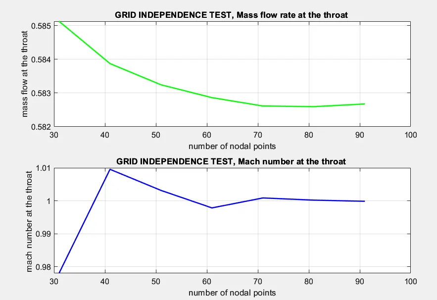
Grid independence test is performed for various values of n for both conservative and non conservative forms and the conclusions are given below
for the Conservative form :
for Non conservative form
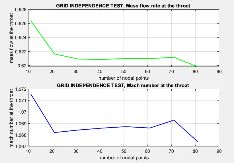
- It can be observed from both the plots that both solutions are grid independent.
- However, the conservative form shows more accurate values as compared to the non conservative form( in comparison to the value obtained from analytical solutions
RESULTS AND DISCUSSION
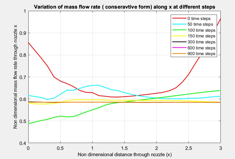
The plots for the mass flow rate along the length of the nozzle for various time steps is plotted for both the conservstive case and the non conservative case
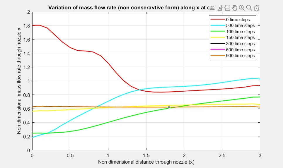
Non conservative (* blue one is the 50th time step and not 500th)
conservative
A few things can be observed from both the plots :
- The mass flow rate in the non-conservation case has higher fluctutation before it comes to a steady state at times steps around 150- 300
- Considering the case of the conservative form , the fluctuation is much lower as the solution approches a steady state around 50 th time step.
- This shows that the conservative form has a faster convergence rate
- Another thing that was noted was that the time taken was way higher for the conservative form.
- Conservation form also gives the mass flow rate value closer to the analytical values of 0.529. The obtained values is around 0.58 for the conservation form whereas its around 0.62 for the non conservative form.
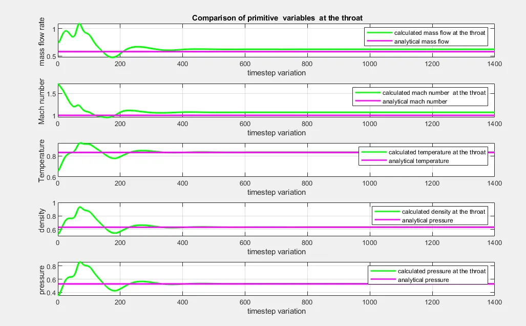
The primitive variable like density, temperature, mach number, velocity, pressure etc are plotted at the throat and the values are given
Non Conservative
Conservative
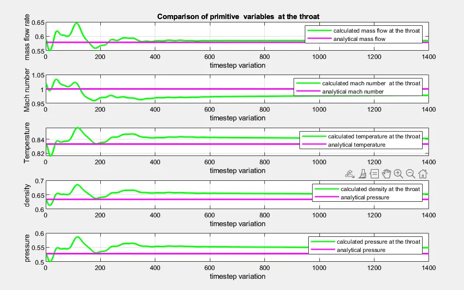
- Certain things can be observed is that the non conservative form is giving more accurate values to the analytical solution as compared to conservative form.
- Also the computational time was much less for the former.
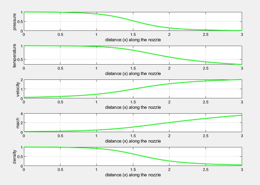
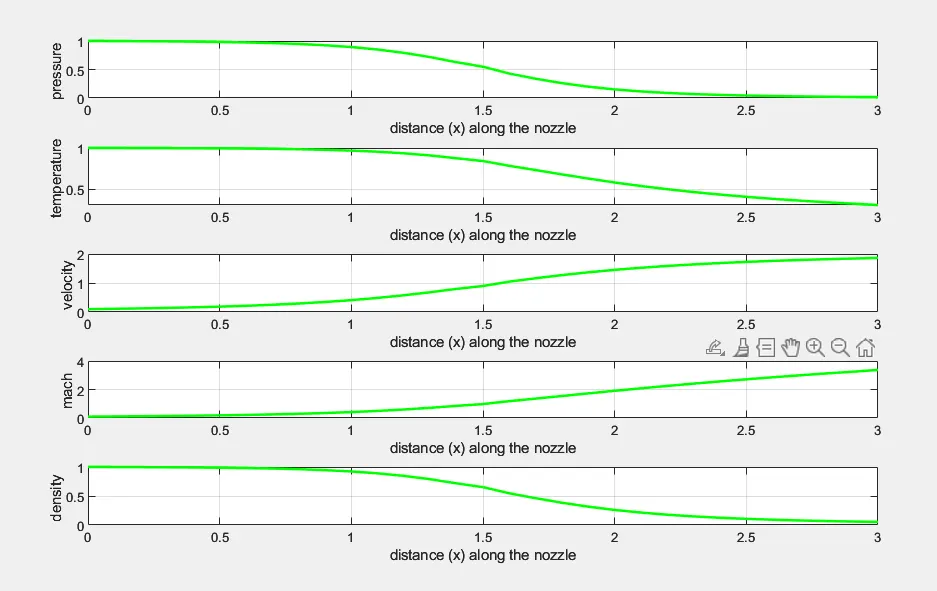
The variation of primitive variables as a function of x is shown in the graphs below :
Non Conservative
Conservative
The normalised mass flow rate is plotted for conservative and non conservative form
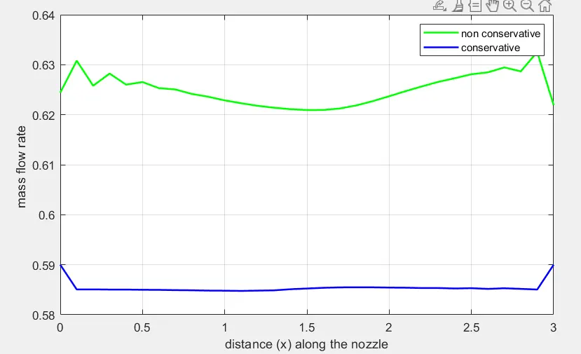
It can be observed from the figure that the conservative form gives a more stable and accurate solution whereas the non conservative form has lots of fluctuations, nevertheless both forms give results which are quite close to the analytical values.
CONCULSION
To conclude, a detailed study has been done using the Maccormack's technique for 1D isentropic con-div nozzle . The analysis was done for both conservative and non conservative forms. Both the methods give results which are quite accurate but there are certain drawbacks for each as the Conservative form takes longer time to solve whereas the non conservative form has more instableness and fluctuations.
On the whole, both are useful, it is just a matter of what to use for which application.
REFERENCES :