Week 7 - Simulation of a 1D Supersonic nozzle flow simulation using Macormack Method
AIM : To simulate the isentropuc flow through a quasi 1D subsonic-supersonic nozzle . to solve both conservation &non-conservation forms of the governing equations by using mac-Cormack's technique. & to determine the steady-state temperature distribution for the flow-field variables and investigate the difference between the two forms of governing equations by comparing solutions.
OBJECTIVE :
- steady-state distribution of primitive variables inside the nozzle.
- time-wise variation of the primitive variables.
- variation of mass flow rate distribution inside the nozzle at different time steps during the time-marching process.
- comparision of normalized mass flow rate distributions of both forms.
THEROY :
a nozzle is a device designed to control the direction or characteristics of a fluid flow (especially to increase velocity) as it exits (or enters) an enclosed chamber or pipe. a nozzle is often a pipe or tube of varying cross-sectional area, and it can be used to direct or modify the flow of a fluid (liquid or gas). nozzles are frequently used to control the rate of flow, speed, direction, mass, shape, and/or the pressure of the stream that emerges from them.there are different types of nozzle but here in our project we uses a convergent divergent nozzle. this nozzle is used to obtain a supersonic stream starting from low speeds at the inlet. then the mach number should increase from ma=0 near the inlet to ma>1 at the exit. it is clear that the nozzle must converge in the subsonic portion and diverge in the supersonic portion. such a nozzle is called a convergent-divergent nozzle.
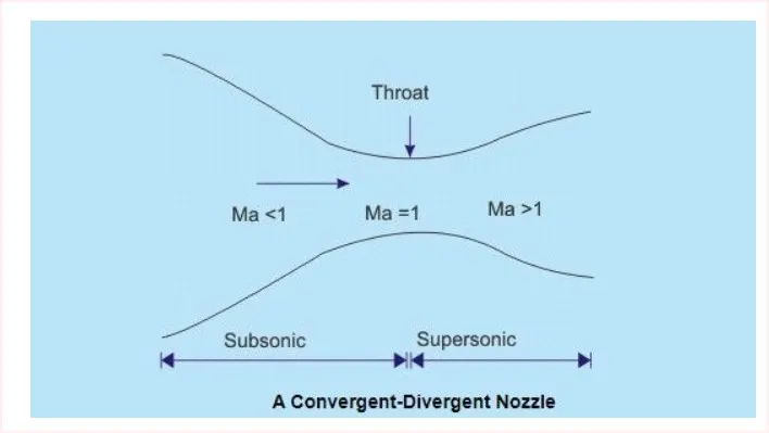
we consider the steady, isentropic flow through a convergent-divergent nozzle. the flow at the inlet to the nozzle comes from a reservoir where pressure and temperatures are at stagnation. also it is assumed that the crosss sectional area of the nozzle is very large so that the velocity is almost v ~ 0. the flow expands adiabatically to supersonic speeds at the nozzle exit. the flow is locally subsonic in the convergent section (m < 1), sonic at the throat section (m = 1) and supersonic at the divergent section ( m> 1).
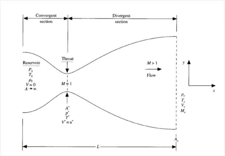
we assume that at a given section, where the cross-sectional area is a, the flow properties are uniform across the section. hence although the area of the nozzle changes as the function of distance along the nozzle x, and therefore in reality the flow field is two-dimensional (the flow varies in two-dimensional x y space), we make the assumption that the flow properties vary only with x; this is tantamount to assuming uniform flow properties across any given cross section. such flow is defined as quasi one-dimensional flow.
MACCORACK'S TECHNIQUE :
Is an explicit finite difference technique which is second order accurate in both space and time .this technique is student friendly and are perfectly satisfactory for many fluid applications it follows three stages of calculations and they are
PREDICTOR STEP :
here we use forward differencing for the space term
CORRECTOR STEP :
backward differencing is used here for the space terms
AVERAGE STEP :
this is simply the average of predictor and corrector step
these will be further clarified for each form.
MAIN CODE :
clear all
close all
clc

n = 31;
x = linspace(0,3,n);
dx = x(2)-x(1);
gamma = 1.4;
nt = 1400;
C = 0.5;
throat = (n-1)/2;
a = (1+2.2*(x-1.5).^2);

tic;
[rho,v,T,P,m,M,T_throat,rho_throat,P_throat,M_throat] = non_conserv(n,x,dx,gamma,nt,C,a,throat);
time_elapsed = toc;
fprintf('computation time = %f',time_elapsed);

time_variation = figure(1);

subplot(4,1,1)
plot(rho_throat,'b')
title('Time-wise variations in quantity in non conservative form');
legend('density')
ylabel('rho/rho_{o}');
grid minor

subplot(4,1,2)
plot(T_throat,'b')
legend('temp')
ylabel('T/T_{o}');
grid minor

subplot(4,1,3)
plot(P_throat,'b')
legend('pressure')
ylabel('p/p_{o}');
grid minor

subplot(4,1,4)
plot(M_throat,'b')
legend('mach no')
grid minor
ylabel('M');
xlabel('no.of iter')

qualitative_non_cons = figure(2);
subplot(4,1,1)
plot(x,M,'b')
title('qualitative aspects of 1D supersonic nozzle:non-conservative form');
ylabel('M')
legend('mach no.')
grid minor

subplot(4,1,2)
plot(x,T,'b')
ylabel('T')
legend('temp')
grid minor

subplot(4,1,3)
plot(x,P,'b')
ylabel('P')
legend('press')
grid minor

subplot(4,1,4)
plot(x,rho,'b')
ylabel('rho')
legend('density')
grid minor

% conservation form
tic
[m_c,v_c,T_c,P_c,M_c,rho_c,T_throat_c,rho_throat_c,P_throat_c,M_throat_c] = conserv_form(x,dx,n,C,a,nt,gamma,throat);
time_elapsed = toc;
time_variation_conser = figure(3);

subplot(4,1,1)
plot(rho_throat_c,'b')
title('Time-wise variations in conservative form');
axis([0 1500 0.6 1.3])
legend('density')
ylabel('rho/rho_{o}');
grid minor

subplot(4,1,2)
plot(T_throat_c,'b')
axis([0 1500 0.6 1])
legend('temp')
ylabel('T/T_{o}');
grid minor

subplot(4,1,3)
plot(P_throat_c,'b')
axis([0 1500 0.4 1.1])
legend('pressure')
ylabel('p/p_{o}');
grid minor

subplot(4,1,4)
plot(M_throat_c,'b')
axis([0 1500 0.6 1.4])
legend('mach no')
ylabel('M');
grid minor
xlabel('no.of iter')

qualitative_cons = figure(4);
subplot(4,1,1)
plot(x,M_c,'b')
title('qualitative aspects of 1D supersonic nozzle flow: Conservative form')
ylabel('M')
legend('mach no.')

subplot(4,1,2)
plot(x,T_c,'b')
ylabel('T/T_{o}');
legend('temp')

subplot(4,1,3)
plot(x,P_c,'b')
ylabel('p/p_{o}');
legend('press')

subplot(4,1,4)
plot(x,rho_c,'b')
ylabel('rho/rho_{o}');
legend('density')

%comparison of mass flow artes by conservative and non-conservative
%methods and comaprison with exact form
mass_comparison = figure(5);
hold on;
plot(x,m_c,'g','LineWidth',1.75);
plot(x,m,'m','LineWidth',1.75);
line([0 3],[0.579 0.579],'LineWidth',1.75);
legend('Conservative Form','Non-Conservative Form','Exact Solution');
grid minor;
xlabel('x/L');
ylabel('rhoVA/rho_{o}V_{o}A_{0}');
title('non-dimensional mass flow comparison with exact solution');
FUNCTION CODE FOR CONSERVATIVE FORM :
function [m_c,M_c,v_c,T_c,P_c,rho_c,T_throat_c,rho_throat_c,P_throat_c,M_throat_c] = conserv_form(x,dx,n,C,a,nt,gamma,throat)

for i = 1:length(x)
    if (x(i) >=0 && x(i) < 0.5)
        rho_c(i) = 1;
        T_c(i) = 1;
    else if (x(i) >= 0.5 && x(i) < 1.5)
            rho_c(i) = 1.0 - 0.366*(x(i) - 0.5);
            T_c(i) = 1.0 - 0.167*(x(i) - 0.5);
        else if (x(i) >= 1.5 && x(i) <= 3)
                rho_c(i) = 0.634 - 0.3879*(x(i) - 1.5);
                T_c(i) = 0.833 - 0.3507*(x(i) - 1.5);
            end
        end
    end
end

v_c = 0.59./(rho_c.*a);
P_c = rho_c.*T_c;

U1 = rho_c.*a;
U2 = rho_c.*a.*v_c;
U3 = rho_c.*a.*((T_c./(gamma-1))+(gamma/2)*(v_c.^2));

for k = 1:1400

    U1_old = U1;
    U2_old = U2;
    U3_old = U3;

     dt = min(C*(dx./(sqrt(T_c)+v_c)));

     F1 = U2;
     F2 = ((U2.^2)./U1)+((gamma-1)/gamma)*(U3 - (gamma*(U2.^2))./(2*U1));
     F3 = ((gamma*U2.*U3)./U1) - (gamma*(gamma-1)/2)*((U2.^3)./(U1.^2));

     for j = 2:n-1

         J2(j) = (1/gamma)*rho_c(j)*T_c(j)*((a(j+1)-a(j))/dx);

         %predictor step
         dU1_dt_p(j) = -(F1(j+1)-F1(j))/dx;
         dU2_dt_p(j) = -((F2(j+1) - F2(j))/dx) + J2(j);
         dU3_dt_p(j) = -(F3(j+1)-F3(j))/dx;

         U1(j) = U1(j) + dU1_dt_p(j)*dt;
         U2(j) = U2(j) + dU2_dt_p(j)*dt;
         U3(j) = U3(j) + dU3_dt_p(j)*dt;
     end

     % updating vriables and flux
      rho_c = U1./a;
         v_c = U2./U1;
         T_c = (gamma-1)*((U3./U1) - (gamma/2)*(v_c.^2));

     F1 = U2;
     F2 = ((U2.^2)./U1)+((gamma-1)/gamma)*(U3 - (gamma*(U2.^2))./(2*U1));
     F3 = ((gamma*U2.*U3)./U1) - (gamma*(gamma-1)/2)*((U2.^3)./(U1.^2));

      for j = 2:n-1

         J2(j) = (1/gamma)*rho_c(j)*T_c(j)*((a(j)-a(j-1))/dx);

         %corrector step
         dU1_dt_c(j) = -(F1(j)-F1(j-1))/dx;
         dU2_dt_c(j) = -((F2(j) - F2(j-1))/dx) + J2(j);
         dU3_dt_c(j) = -(F3(j)-F3(j-1))/dx;
      end

      %updating the sol
      %avg val
      dU1_dt = 0.5*(dU1_dt_p + dU1_dt_c);
       dU2_dt = 0.5*(dU2_dt_p + dU2_dt_c);
       dU3_dt = 0.5*(dU3_dt_p + dU3_dt_c);

       % final sol update
       for i = 2:n-1
           U1(i) = U1_old(i) + dU1_dt(i)*dt;
            U2(i) = U2_old(i) + dU2_dt(i)*dt;
             U3(i) = U3_old(i) + dU3_dt(i)*dt;
       end

       % flow field variables update
         rho_c = U1./a;
         v_c = U2./U1;
         T_c = (gamma-1)*((U3./U1) - ((gamma/2)*(v_c.^2)));

       %boundary cond
       %inlet
       U1(1) = rho_c(1)*a(1);
       U2(1) = 2*U2(2) - U2(3);
       U3(1) =  U1(1)*((T_c(1)/(gamma-1))+(0.5*gamma*(v_c(1)^2)));


       %outlet
    U1(n) = 2*U1(n-1) - U1(n-2);
    U2(n) = 2*U2(n-1) - U2(n-2);
    U3(n) = 2*U3(n-1) - U3(n-2);


         % p,mach,mass
         P_c = rho_c.*T_c;
         M_c = v_c./(sqrt(T_c));
         m_c = rho_c.*a.*v_c;

         % @throat
         M_throat_c(k) = M_c(throat);
         P_throat_c(k) = P_c(throat);
         T_throat_c(k) = T_c(throat);
         rho_throat_c(k) = rho_c(throat);

         %comparison of non-dimensional mass flow rates at diffferent
         %times:
         mass2 = figure(7);
         hold on;
         if k ==100
             plot(x,m_c,'b','linewidth',1.75);
         else if k ==200
                 plot(x,m_c,'g','linewidth',1.75);
             else if k ==700
                     plot(x,m_c,'r','linewidth',1.75);
                 end
             end
         end
end
title('Comparison of non-dimensional mass flow rates at different time-instants(conservative form');
xlabel('x/L (Non-dimensional distance through the nozzle)');
ylabel('rhoVA/rho_{o}V_{o}A_{o}');
legend('1000Deltat','200Deltat','700Deltat');
axis([0 3 0.4 1.6]);
grid on;
grid minor;
end
FUNCTION CODE FOR NON-CONSERVATIVE FORM :
function [rho,v,T,P,m,M,T_throat,rho_throat,P_throat,M_throat] = non_conserv(n,x,dx,gamma,nt,C,a,throat)


rho = 1-0.3146*x;
T = 1-0.2314*x;
v = (0.1+1.09*x).*T.^0.5;

for k = 1:nt

    rho_old = rho;
    v_old = v;
    T_old = T;

    dt = min(C.*dx./(sqrt(T)+v));

    % predictor method

    for j = 2:n-1

        dv_dx = (v(j+1)-v(j))/dx;
        drho_dx = (rho(j+1)-rho(j))/dx;
        dT_dx = (T(j+1)-T(j))/dx;
        dloga_dx = (log(a(j+1))-log(a(j)))/dx;

        % continuity eq
        drho_dt_p(j) = -rho(j)*dv_dx-rho(j)*v(j)*dloga_dx-v(j)*drho_dx;

        %momentum eq
        dv_dt_p(j) = -v(j)*dv_dx-(1/gamma)*(dT_dx+(T(j)/rho(j))*drho_dx);

        % energy eq
        dT_dt_p(j) = -v(j)*dT_dx-(gamma-1)*T(j)*(dv_dx+v(j)*dloga_dx);

        % solution update
    rho(j) = rho(j) + drho_dt_p(j)*dt;
    v(j) = v(j) + dv_dt_p(j)*dt;
     T(j) = T(j) + dT_dt_p(j)*dt;

    end


% corrector method

    % continuity eq

    for j = 2:n-1

        dv_dx = (v(j)-v(j-1))/dx;
        drho_dx = (rho(j)-rho(j-1))/dx;
        dT_dx = (T(j)-T(j-1))/dx;
        dloga_dx = (log(a(j))-log(a(j-1)))/dx;

        % continuity eq
        drho_dt_c(j) = -rho(j)*dv_dx-rho(j)*v(j)*dloga_dx-v(j)*drho_dx;

        %momentum eq
        dv_dt_c(j) = -v(j)*dv_dx-(1/gamma)*(dT_dx+(T(j)/rho(j))*drho_dx);

        % energy eq
        dT_dt_c(j) = -v(j)*dT_dx-(gamma-1)*T(j)*(dv_dx+v(j)*dloga_dx);

    end


    % compute the average time derivative

    drho_dt = 0.5*(drho_dt_p+drho_dt_c);
    dv_dt = 0.5*(dv_dt_p+dv_dt_c);
    dT_dt = 0.5*(dT_dt_p+dT_dt_c);

    % final solution update

    for i = 2:n-1
    rho(i) = rho_old(i) + drho_dt(i)*dt;
    v(i) = v_old(i) + dv_dt(i)*dt;
    T(i) = T_old(i) + dT_dt(i)*dt;
    end

    % apply boundary conditions
    %inlet
    v(1) = 2*v(2)-v(3);
    rho(1) = 1;
    T(1) = 1;

    %outlet
    rho(n) = 2*rho(n-1)-rho(n-2);
    v(n) = 2*v(n-1)-v(n-2);
    T(n) = 2*T(n-1)-T(n-2);

  % defining the values for p,m,
  P = rho.*T;
  m = rho.*a.*v;
  M = v./sqrt(T);

  % @throat
  T_throat(k) = T(throat);
  P_throat(k) = P(throat);
  rho_throat(k) = rho(throat);
  M_throat(k) = M(throat);

% comparison of non-dimensional mass flow rates at different times:
mass = figure(6);
hold on;
if k == 50
    plot(x,m,'b','linewidth',1.75);
else if k == 100
        plot(x,m,'g','linewidth',1.75);
    else if k == 150
            plot(x,m,'r','linewidth',1.75);
        else if k == 200
                plot(x,m,'m','linewidth',1.75);
            else if k == 700
                    plot(x,m,'-','linewidth',1.75);
                    plot(x(end),m(end),'b*');
                end
            end
        end
    end
end
end

title('Comparison of non-dimensional mass flow rates at different time-instants');
xlabel('x/L (Non-dimensional distance through the nozzle)');
ylabel('rhoVA/rho_{o}V_{o}A_{o}');
legend('50Deltat','100Deltat','150Deltat','200Deltat','700Deltat');
axis([0 3 0 2.5]);
grid on;
grid minor;
end
RESULTS :
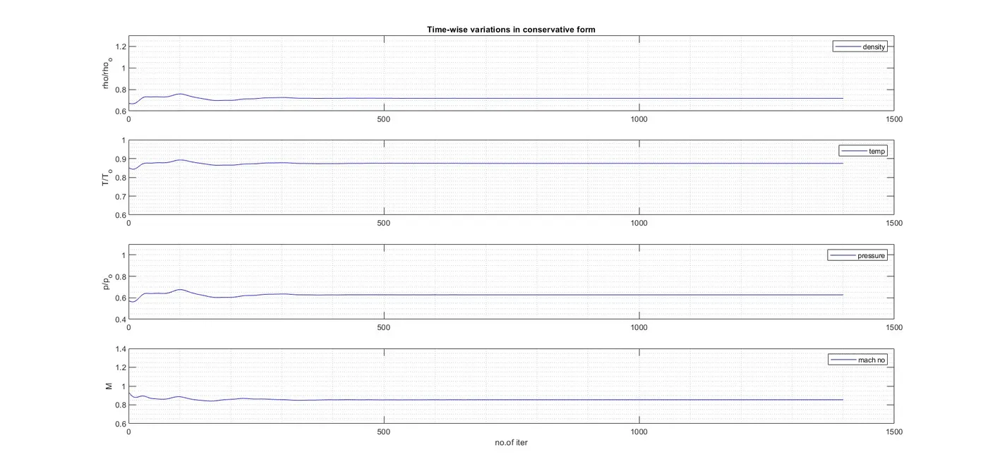
1.TIME-WISE VARIATION OF PRESSURE,TEMPERATURE,VELOCITY &MACH NUMBER AT NOZZLE THROAT :
conservative form :
non-conservative form :
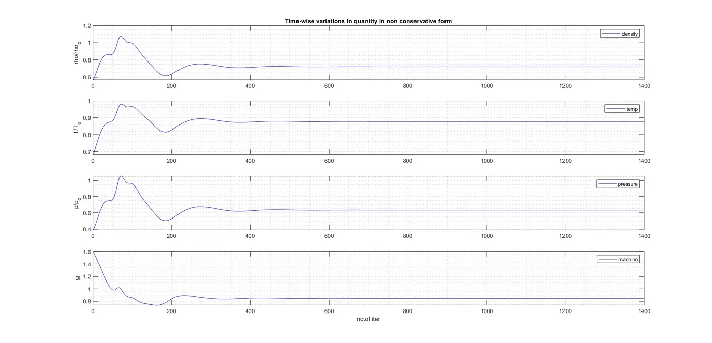
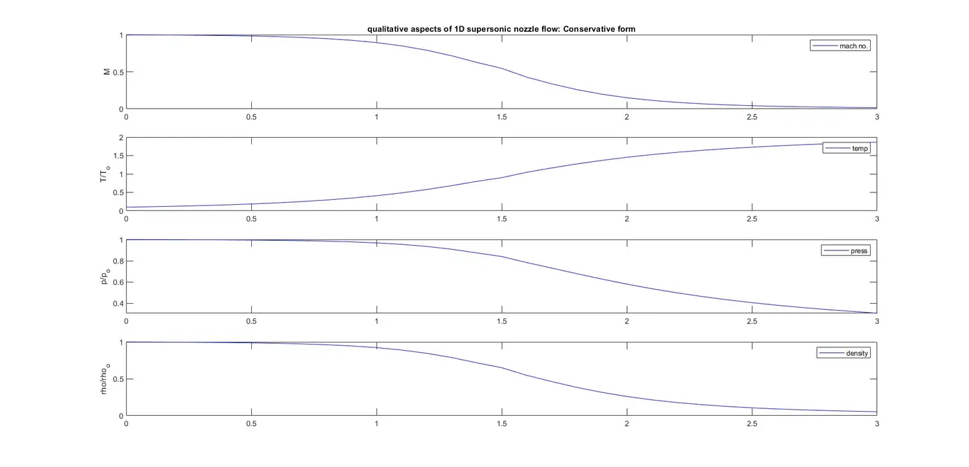
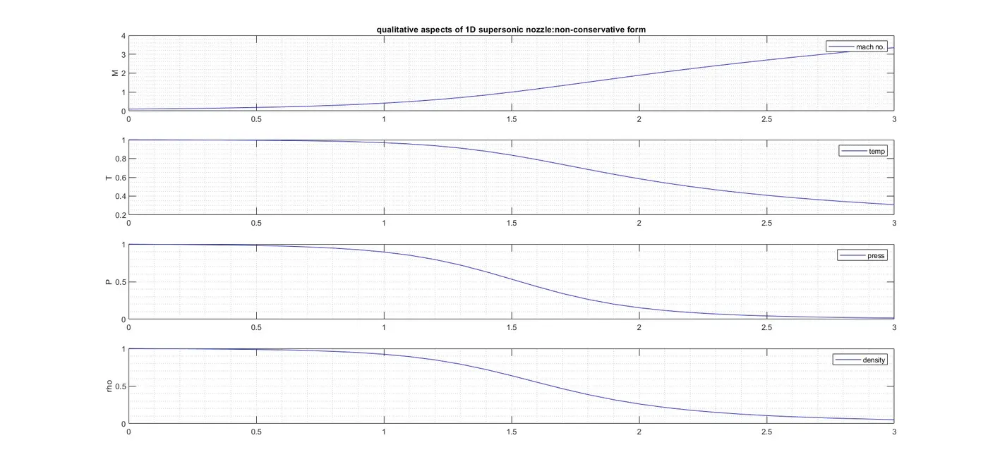
2.QUALITATIVE ASSPECTS OF QUASI 1D NOZZLE FLOW AT STEADY STATE :
conservative form :
non-conservative form :
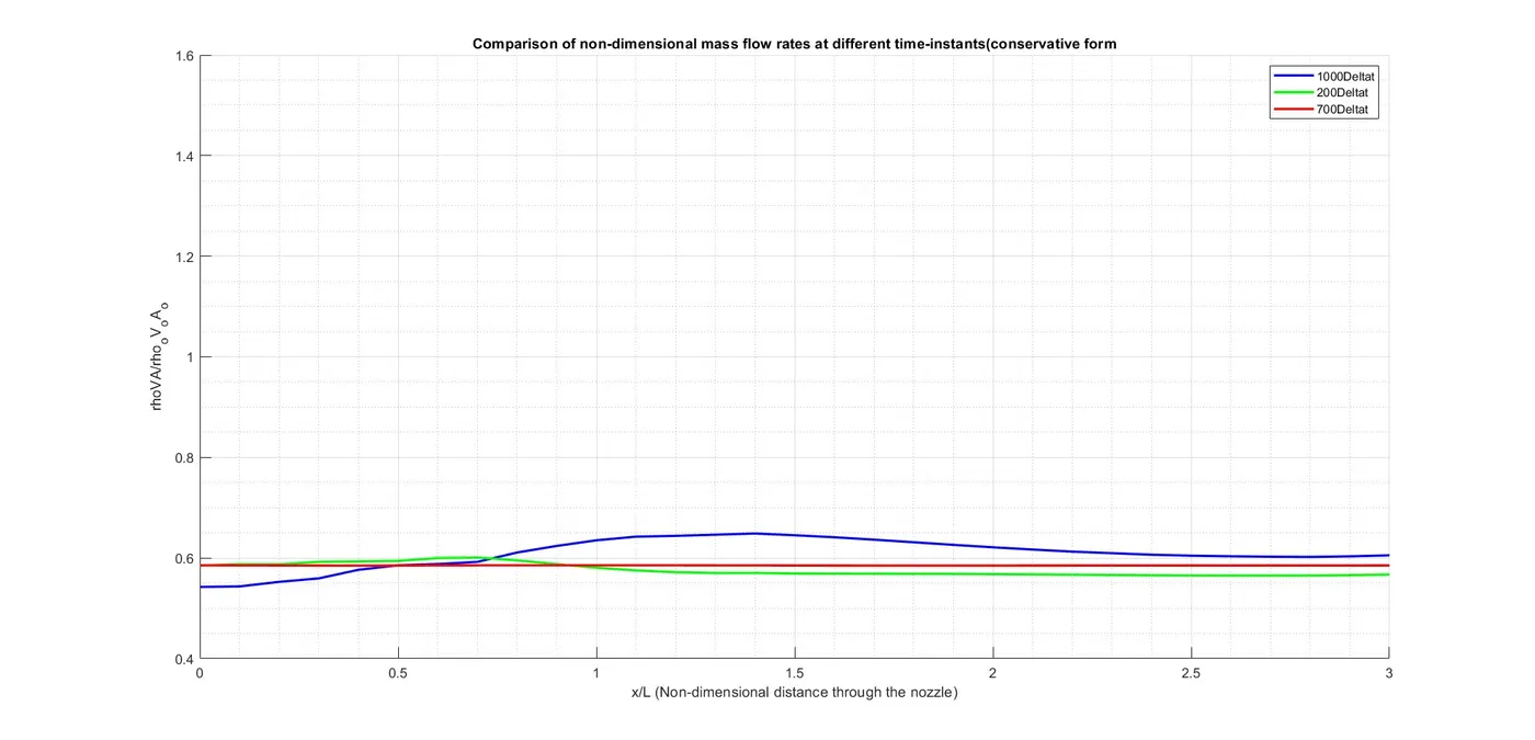
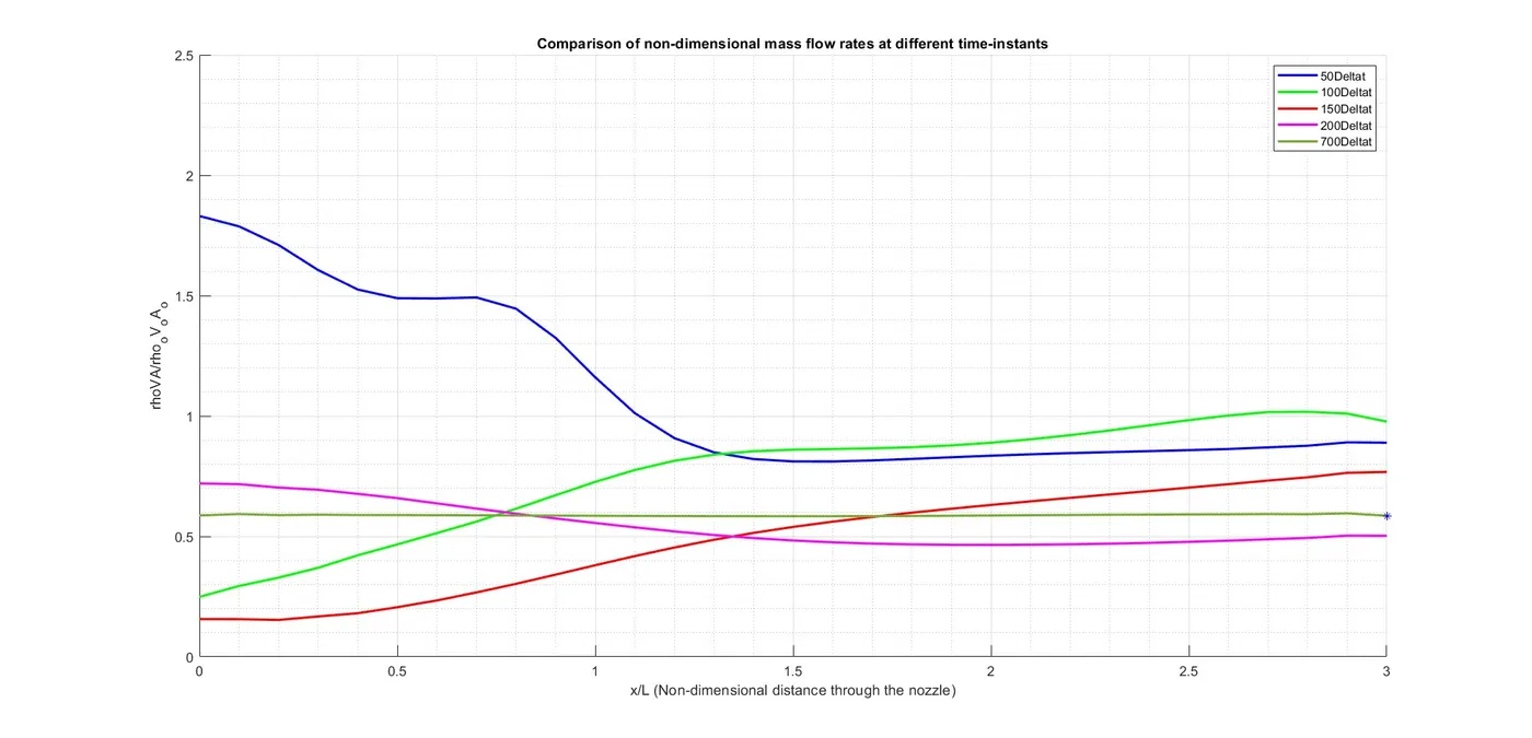
3.NON-DIEMENSIONAL MASS FLOW RATE DISTRIBUTION AT VARIOUS TIME STEPS :
conservative form :
non-conservative form :
4.COMNPARISION OF NON-DIEMENSIONAL MASS FLOW RATES OF BOTH FORMS :
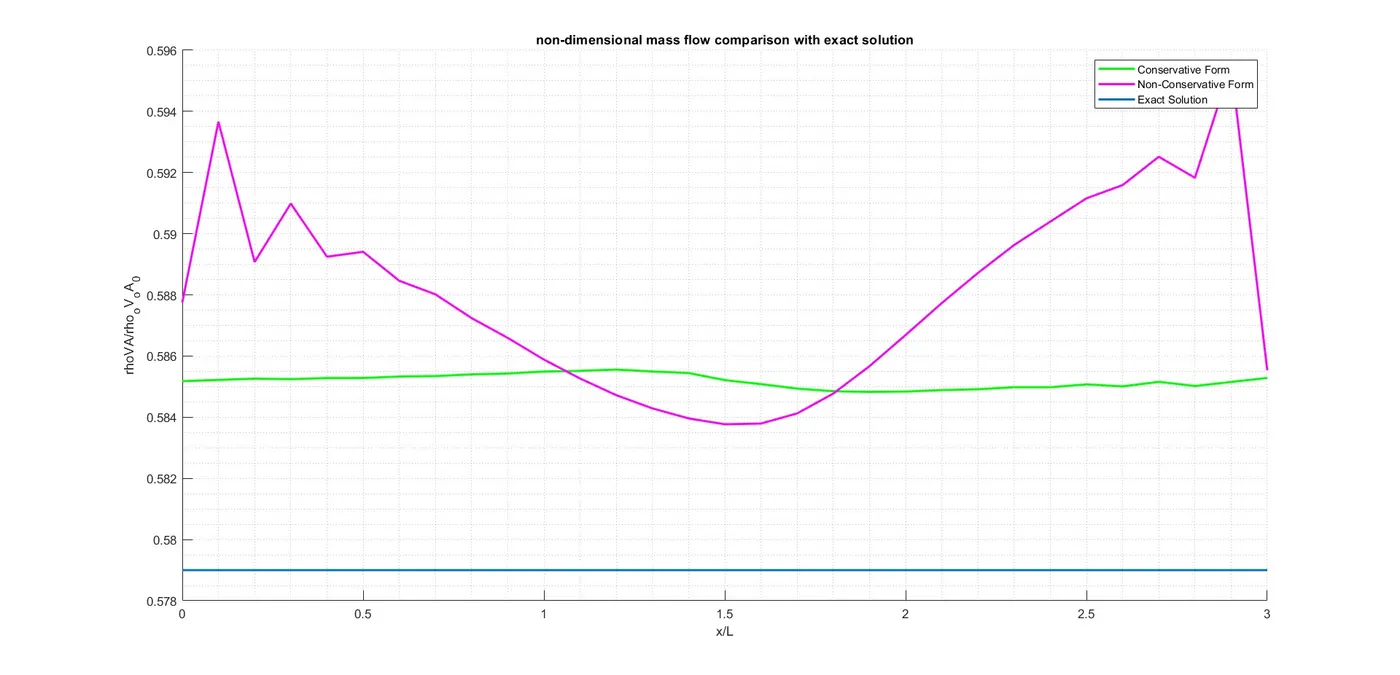
as evident from the plot the conservative form gives a mass flow rate variation that is close to a constant value and simultaneously close to the exact value of 0.579 at the steady state .the non-conservative form shows some oscillations around the inflow and outflow boundaries and is less satisfactory compared to the conservation form.
this project investigates a compressible, steady, isentropic flow through convergent-divergent nozzle. the physics modelled in the code is massively simplified by assuming that the flow field variables change only with 'x' (thereby making it quasi 1 dimensional). the problem has been modelled by numerically solving both the conservative and non-conservative forms of the governing equations that have been discretised by McCormack’s method. despite being mathematically equivalent, on numerically solving both these forms, the obtained graphs for the mass flow rates at steady state show small variations. the graphs showing the variables changing with the time-steps are also slightly different for the conservative and non-conservative forms. however, the steady state distributions for the flow field variables (density, velocity and temperature) obtained from both forms are the same. increasing the mesh fineness increases the accuracy of the results but imposes a higher computational cost.
GRID-INDEPENDENCE TEST :
| p/p0 | T/T0 | p/p0 | M | |
| exact analytical solution | 0.634 | 0.833 | 0.528 | 1.000 |
| conservative form [n=31] | 0.6504 | 0.8400 | 0.5464 | 0.9817 |
| non-conservative form [n=31] | 0.6387 | 0.8365 | 0.5342 | 0.9994 |
| conservative form [n=61] | 0.6382 | 0.8352 | 0.5330 | 0.9993 |
| non-conservative form[n=61] | 0.6376 | 0.8354 | 0.5326 | 0.9997 |
from the above results we can see that for a grid-size of 30 points the non-conservative form gives a more accurate result compared to the conservative form. however, when we change the grid-size to 60 points the values of the flow quantities are quite close when calculated by either of the methods. additionally, both the methods give results which are closer to the exact value in this case.