Week 3 - Solving second order ODEs

The ODE for simple pendulum considering damping is given as :

d2θdt2+(bm)⋅dθdt+(gl)⋅sin(θ)=0">d2θdt2+(bm)⋅dθdt+(gl)⋅sin(θ)=0d2θdt2+(bm)⋅dθdt+(gl)⋅sin(θ)=0

we cannot solve 2nd order ode in matlab hence we have to convert it into 1st order ode first and then perform the operation.

considering, θ=θ1(displacement)

dθ/dt=dθ1/dt=θ2(velocity)

d^2θ/dt^2=d^2θ1/dt^2=dθ2/dt

hence on substituting the above equation in our given ode

we get; dθ2/dt+(b/m)*θ2+(g/l)*sin(θ1)=0

we get a 2*1 matrix to solve for second order ode

theta1_dt=dθ1/dt=θ2

theta2_dt=dθ2/dt= -(b/m)*θ2+(g/l)*sin(θ1)

g = gravity in m/s2,

L = length of the pendulum in m,

m = mass of the ball in kg,

b=damping coefficient.

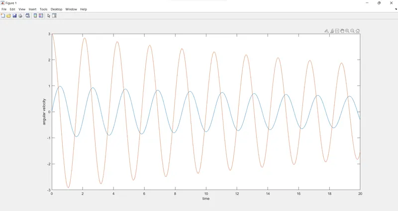
here we have the intial conditions and time and plots for figure 1 and xlabel for time and ylabel for angular velocity when the damping increases the resistances also increased and velocity of sphere ball decreased

here we have the plots for to create the fixed beam,pendulum line and ball position,and getting frames and counter increment,and making movie creation and animation

following is the main code

% Program to solve 2nd order ODE for pendulum
close all
clear all
clc

% inputs 

% length of pendulum (m)
l=1;    
% mass of ball (kg)
m=1;    
% Damping Coefficient
b=0.05; 
% gravitational acceleration(m/s^2)
g=9.81; 

% Initial Condition
theta_0 = [0;3];

% time points
t_span = linspace(0,20,300);

% ode solution
[t results] = ode45(@(t,theta) ode_func(t, theta, b, g, l, m), t_span, theta_0);

% plot results
figure(1)
plot(t, results(:,1))
hold on
plot(t, results(:,2))
xlabel('time')
ylabel('angular velocity')

ct = 1;		
for i = 1 : length(results(:,1))
    
    x0 = 0;
    y0 = 0;
    x1 = l*sin(results(i,1));
    y1 = -l*cos(results(i,1));
    figure(2)
    % plot fixed support
    plot([-1 1], [0 0], 'linewidth', 10, 'color', 'b')		
    axis([-2 2 -2 2])
    hold on
    % plot string position
    line([x0 x1], [y0 y1], 'linewidth', 5, 'color', 'y')
    % plot ball position
    plot(x1, y1, 'o', 'markersize', 25, 'markerfacecolor', 'r')
    hold off
    M(ct) = getframe(gcf);	
    ct = ct+1;
end

movie(M)
videofile = VideoWriter('Pendulum_simulation.avi', 'Uncompressed AVI');
open(videofile)
writeVideo(videofile, M)
close(videofile)		

















FUNCTION

function [dtheta_dt] = ode_func(t, theta, b, g, l, m)

theta1 = theta(1);
theta2 = theta(2);
dtheta1_dt = theta2;
dtheta2_dt = -(b/m)*theta2 - (g/l)*sin(theta1);
dtheta_dt = [dtheta1_dt; dtheta2_dt];
end

we have made use of function as we have 2 odes to solve hence we have not used only inbuilt function for ode45

LINK :

https://youtu.be/X9Yud0quryQ

The plot between between time period(t) with respect to displacement and velocity shows the daming effect and change in magnitude of velocity and displacement as time t increases along x- axis.

We have created animation using inbuilt functions to keep track of image generated for each value of t and storing them the inbuilt function imwrite stores the images and then creates a animation.