Week 5 - Genetic Algorithm

INTRODUCTION OF GA:

a genetic algorithm (ga) is a method for solving both constrained and unconstrained optimization problems based on a natural selection process that mimics biological evolution. the algorithm repeatedly modifies a population of individual solutions. at each step, the genetic algorithm randomly selects individuals from the current population and uses them as parents to produce the children for the next generation. over successive generations, the population "evolves" toward an optimal solution.you can apply the genetic algorithm to solve problems that are not well suited for standard optimization algorithms, including problems in which the objective function is discontinuous, nondifferentiable, stochastic, or highly nonlinear.the genetic algorithm differs from a classical, derivative-based, optimization algorithm in two main ways

SYNTAX FOR GA:

• start
• x=ga(@fun,nvars,a,b,aeq,beq,lb,ub,nonlcon,intcon,options)
• fun= the fitness function in our case the stalagmite function.
• nvars= number of variables (2)
• a and b= linear inequalities of the form a*x<=b
• aeq and beq=linear equalities of the form a*x=b
• lb and ub=lower and upper bound that is the region in which ga will search for the result.
• nonlcon=non linear inequalities
• intcon=integer constrained
• options= helps to add constrain tolerance by increasing the population size.
• for our first case, all the above options are not used so ga will assume the default values.
• subplot(2,1,1)
• surfc(xx,yy,-f)
• hold on
• shading interp
• plot3(xopt,yopt,-fopt,'marker','o','markersize',5,'markerfacecolor','r')
• title('unbounded inputs')
• xlabel('x-axis')
• ylabel('y-axis')
• subplot(2,1,2)
• plot(fopt)
• xlabel('iterations')
• ylabel('function maxima')
• end
• we will be creating two plots so we will be applying the subplot command. the surfc is used to view the 3-d graph of the points xx,yy,-f, here the -f is to represent the graph in the positive axis. hold on is used to views all the plots. sharp interp is used so that the 3-d graph is more representable.
• plot 3 is used to plot all the three values xopt,yopt and -fopt in the 3-graph and the second subplot only views the fopt in a 2-d graph.

clear all
close all
clc

x=linspace(0,0.6,150);
y=linspace(0,0.6,150);
num_cases=50
[xx, yy]=meshgrid(x, y);

for i=1:length(xx)
    for j=1:length(yy)
        input_vector(1)=xx(i,j);
        input_vector(2)=yy(i,j);
        F(i,j)=stalagmite(input_vector);
      end 
end

%Study 1- Statistical behaviour
tic
for i=1:num_cases
    [inputs, fopt(i)]=ga(@stalagmite,2);
    xopt(i)=inputs(1);
    yopt(i)=inputs(2);
end

study1_time=toc
%unbounded inputs
figure(1)
subplot(2,1,1)
surfc(xx,yy,-F)
hold on
shading interp
plot3(xopt,yopt,-fopt,'marker','o','markersize',5,'markerfacecolor','r')
title('Unbounded inputs')
xlabel('X-axis')
ylabel('Y-axis')
subplot(2,1,2)
plot(fopt)
xlabel('Iterations')
ylabel('Function Maxima')

%Study-2(Statistical behavior-With Upper and Lower bounds)
tic
for i=1:num_cases
    [inputs, fopt(i)]=ga(@stalagmite,2,[],[],[],[],[0;0],[0.5;0.5]);
    xopt(i)=inputs(1);
    yopt(i)=inputs(2);
end
study2_time=toc 
%bounded inputs
figure(2)
subplot(2,1,1)
surfc(xx,yy,-F)
hold on
shading interp
plot3(xopt,yopt,-fopt,'marker','o','markersize',5,'markerfacecolor','r')
title('Bounded inputs')
xlabel('X-axis')
ylabel('Y-axis')
subplot(2,1,2)
plot(-fopt)
xlabel('Iterations')
ylabel('Function Maxima')

%Study 3 Incresing the GA Iteration
options=optimoptions('ga');
options=optimoptions(options,'PopulationSize',200);

tic
for i=1:num_cases
    [inputs, fopt(i)]=ga(@stalagmite,2,[],[],[],[],[0;0],[0.5;0.5],[],[],options);
    xopt(i)=inputs(1);
    yopt(i)=inputs(2);
end
study3_time=toc
%optimisation
figure(3)
subplot(2,1,1)
surfc(xx,yy,-F)
hold on
shading interp
plot3(xopt,yopt,-fopt,'marker','o','markersize',5,'markerfacecolor','r')
title('bounded inputs with Population as 250')
xlabel('X-axis')
ylabel('Y-axis')


subplot(2,1,2)
plot(-fopt)
xlabel('Iterations')
ylabel('Function Maxima')

STALAGMITE FUNCTION:

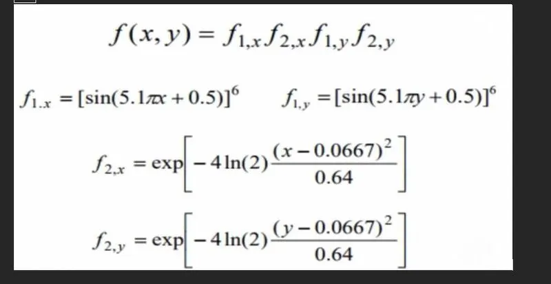
a stalagmite is an upward-growing mound of mineral deposits that have precipitated from water dripping onto the floor of a cave. the figures we get is in the shape of stalagmite so we use this name here. these formulas are represented in the below .

function[F]=stalagmite(input_vector)
x=input_vector(1);
y=input_vector(2);
f1=(sin(5.1*pi*x+0.5))^6;
f2=(sin(5.1*pi*y+0.5))^6;
f3=exp(-4*log(2)*((x-0.0667)^2/0.64));
f4=exp(-4*log(2)*((y-0.0667)^2/0.64));
F=f1*f2*f3*f4*-1;
end

RESULTS:

CASE 3:

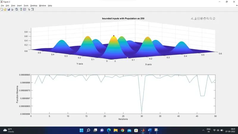
In this case study, we will be increasing the population number from 50 which is the default value a to 200. The higher the number of the population it increases the probability of us finding the optimum function.

There are several things to be kept in mind when dealing with GA population −

• The diversity of the population should be maintained otherwise it might lead to premature convergence.

• The population size should not be kept very large as it can cause a GA to slow down, while a smaller population might not be enough for a good mating pool. Therefore, an optimal population size needs to be decided by trial and error.

So in this case the Population is 200 and the other values are the same as of the second case study. So the time taken to run the program will be more for this case.

You can see from that the options command is used to provide the value of the population. The optimoptions command is used to create the optimization options for the Ga algorithm and the population size is inputted.

CASE 2:

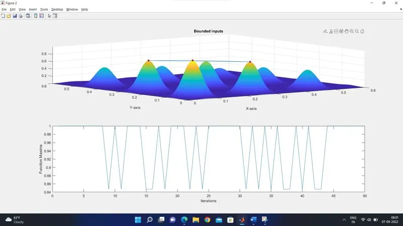
Since we are able to see the Surface graph from the first study we can assume where the Maximum will be hence so we will be directing the algorithm to search in that region.

Only this region of the code will be modified in the second case study. You can see that we are giving the upper and lower bounds value (0,0) and (.5,.5). We are instructing the algorithm that the maximum will be under that region. The Population for this study will be 50 which is the default value.

CASE 1:

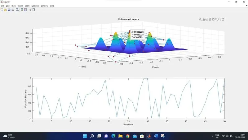
For the first case study, we will be running the Ga algorithm without any bounds Lower bound or Upper bound and the default population 50. And since Ga is an iterative solver the loop is fun for 50 loops.

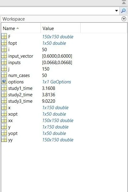
The inputs have two values the x and y coordinate of the fopt. we can see that the stalagmite function is used and the variable two are inputted. The xopt is the "x" value from the input and yopt is the "y" value. And we will be calculating the time taken using the tic and toc commands

CONCLUSION:

In this challenge, the concept of a Genetic algorithm was used to optimize the stalagmite function to find the Global maxima. The concept and working of genetic algorithm are studied and used in the three cases to optimize the function and find the Global maxima.