Week 7 - Simulation of a 1D Supersonic nozzle flow simulation using Macormack Method
Objective
To simulate the isentropic flow through a quasi 1D subsonic - supersonic nzzle for both conservative and non - conservative forms of goverrning equations using MacCormack's technique.
Theory
Consider a steady state isentropic flow through a convergent-divergent nozzle as shown in below figure.
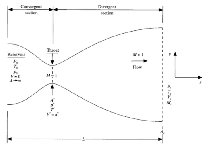
The inlet is connected to a large reservoir, with initial parameters as pressure (Po) and temperature (To). Since the area of the reservoir is assumed to be infinity, initial velocity Vo is very small, almost 0. Also, it is a subsonic region, hence, Mach number M is less than1. The flow undergoes isentropic expansion, and reaches supersonic condtion M>1 at the exit with Pe, Te, Ve and Ae as the parameters. At the throat section, sonic flow is assumed (M=1), and hence, the flow velocity is equal to the speed of sound at this region, denoted by a*, area A*, pressure P* and Temperature T*.
There are mainly two assumptions considered in this case:
- At a given cross sectional are A, the flow properties are uniform.
- Even though the area changes with distance x and the flow properties are 2 dimensional, we assume 1- directional flow properties, thus called as quasi-one-dimensional flow.
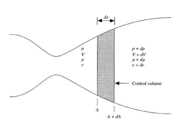
Assume a small control volue with parameters as shown in the above figure.
The governing equations that define the flow are continuity, momentum and energy equations.
- The non conservative form of governing equations which are non non dimensional are
- Continuity equation
`(∂p)/(∂t) = -ρ*(∂v)/(∂x)-rho*V*(∂(lnA))/(∂x)-V*(∂rho)/(∂x)`
- Momentum equation
`(∂v)/(∂t) = -v*(∂v)/(∂x)- (1/gamma)*((∂t)/(∂x) + T/rho*(∂rho)/(∂x))`
- Energy equation
`(∂T)/(∂t) = -V*((∂T)/(∂x)) - (gamma-1)*T*((∂v)/(∂x)+V*(∂(lnA))/(∂x))`
Where `gamma` is the ratio of specific heats `(Cp)/(Cv)` and is 1.4 for standard air conditions.
Initial conditions :
nozzle area, `A=1+2.2*(x-1.5)^2` ; 0 `<=` x `<=` 3
velocity , ` v= (0.1 + 1.09*x)*T^(1/2)`
density , `rho = 1-0.3146*x`
Temperature, `T = 1-0.2314*x`
The conservative form of governing equations, which are non dimensional are
- Continuity Equation
`(∂(rhoA))/(∂t) + (∂(rhoAv))/(∂x)=0`
- Momentum Equation
`(∂(rhovA))/(∂t) + (∂(rhoV^2A+(1/gamma)*rho*A))/(∂x) = (1)/(gamma)*rho*(∂A)/(∂x)`
- Energy Equation
`(∂(rho*((e/(gamma-1))+(gamma/2)*v^2)*A))/(dt) + (∂(rho*(e/(gamma-1)+gamma/n*V^2)*vA+rhovA))/(∂x) = 0`
These equations can be written as
`(∂U1)/(∂t) + (∂F1)/(∂x) = 0 ` -- continuity equation
`(∂U2)/(∂t) + (∂F2)/(∂x) = J2` -- momentum equation
`(∂U3)/(∂t) + (∂F3)/(∂x) = 0 ` -- energy equation
Where U1, U2, and U3 are called as the solution vectors; F1,F2 and F3 are the flux vectors; and J is the source term.
| Solution terms | Flux Terms | Source terms |
| `U1 = rhoA` | `F1 = rhoAv` | |
| `U2 = rhoAv` | `F2 = rhov^2A+1/gamma*rhoA` | `J2 = 1/gamma*rho*(∂A)/(∂x)` |
|
`U3 = rho*(e/(gamma-1)+gamma/2*v^2)*A` |
`F3 = rho*(e/(gamma-1)+gamma/2*v^2)*vA +rhovA` |
Inorder to avoid difficulties during computation and calculations, the flux vectors are represented in terms of solution vectors, i.e,
F1=F1(U1,U2,U3)
F2=F2(U1,U2,U3)
F3=F3(U1,U2,U3)
J2=J2(U1,U2,U3)
where,
`F1=U2`
`F2= ((U2)^2)/(U1) + (gamma-1)/gamma*(U3-gamma/2*((u2)^2)/(u1))`
`F3=(gamma*U2*U3)/(U1)-(gamma*(gamma-1))/2*(((U2)^3))/((u1)^2)`
`J2=(gamma-1)/gamma*(U3-gamma/2*((U2)^2)/(U1))*(∂(lnA))/(∂x)`
Initial conditions :
Nozzle area, `A = 1+2.2*(x-1.5)^2; 0<=x<=3`
Velocity , `v = (U2)/(rhoA) = (0.59)/(rhoA)`
`0<=x<=0.5; {(rho=1),(T=1):}`
`0.5<=x<=1.5; {(rho = 1-0.366*(x-0.5)),(T=1-0.167*(x-0.5)):}`
`1.5<=x<=3; {(rho=0.634-0.3879*(x-1.5)),(T=0.833-0.3507*(x-1.5)):}`
Calculation of Time Step-Adaptive Time Step Method
`dt(i) = CFL* (dx)/(ai + vi)`
`dt = min(dt(i))`
where a is the local speed of sound, `a = sqrt(T)`
These equations are solved by the MacCormack's technique
Assume f(x) as the function to be solved. Solving this using MacCormack's technique involves
Initial profile : Here, certain initial assumptions are considered for the flow field variables.
Predicted step : forward differencing scheme is applied on the spatila terms, and obtaining the predicted derivatives,
`(∂f)/(∂tp) = (f(i+x)-f(i))/(Δx)`
with these predicted time derivatives, we update the initial conditions.
`f = fi + (∂f)/(∂tp)*dt`
corrcected step : here, backward differencing is employed for the spatial terms
`(∂f)/(∂tc) = (f(i)-f(i-1))/(Deltax)`
it is of immense importance to use the updated values of initial condition from the predicted step.
Average step : here we compute the average values of time derivatives from predicted and corrected time steps
`(∂f)/(∂tavg) = 0.5*((∂f)/(∂tp) + (∂f)/(∂tc))`
Final solution update;
`f = fi + (∂f)/(∂tavg)*dt`
Code
Main Program
-
clear allclose allclc%creating x meshn=31;x=linspace(0,3,n);dx=x(2)-x(1);CFL=0.5;throat=(n+1)/2;%areaa=1+2.2*(x-1.5).^2;%initial profile[m_dot_throat_nc,M_throat_nc,T_throat_nc,P_throat_nc,rho_throat_nc,t,M_nc,P_nc,rho,v,m_dot_nc]=non_conservative(n,x,dx,throat,a,CFL);[m_dot_throat,M_throat,T_throat,P_throat,rho_throat,t,M,P,rho,v,m_dot]=conservative(n,x,dx,throat,a,CFL)%COMPARISON GRAPHSfigure(1)hold onplot(x,m_dot,'-*')plot(x,m_dot_nc,'-*')ylim([0.575 0.62])set(gca,'YTick',(0.575:0.005:0.62))xlabel('x')ylabel('mass flow rate')legend('conservative','non-conservative')title('mass flow rate- conservative vs non-conservative')grid onfigure(2)hold onplot(M_throat,'linewidth',0.95)plot(M_throat_nc,'linewidth',0.95)xlabel('timesteps')ylabel('mach number')legend('conservative','non-conservative')title('mach number variation at throat for conservative and non-conservative')figure(3)hold onplot(T_throat,'linewidth',0.95)plot(T_throat_nc,'linewidth',0.95)xlabel('timesteps')ylabel('Temperature')legend('conservative','non-conservative')title('Temperature variation at throat for conservative and non-conservative')figure(4)hold onplot(P_throat,'linewidth',0.95)plot(P_throat_nc,'linewidth',0.95)xlabel('timesteps')ylabel('Pressure')legend('conservative','non-conservative')title('Pressure variation at throat for conservative and non-conservative')figure(5)hold onplot(rho_throat,'linewidth',0.95)plot(rho_throat_nc,'linewidth',0.95)xlabel('timesteps')ylabel('Density')legend('conservative','non-conservative')title('Density variation at throat for conservative and non-conservative')%Non conservative formfigure(6)subplot(4,1,1)plot(x,t,'-*')xlabel('x-distance')ylabel('temperature ratio')title('Flow parameters -non-conservative form')subplot(4,1,2)plot(x,M_nc,'-*')xlabel('x-distance')ylabel('mach number')subplot(4,1,3)plot(x,P_nc,'-*')xlabel('x-distance')ylabel('pressure ratio')subplot(4,1,4)plot(x,rho,'-*')xlabel('x-distance')ylabel('density ratio')figure(7)hold onplot(x,t,'linewidth',0.95)plot(x,rho,'linewidth',0.95,'color','r')plot(x,v,'linewidth',0.95,'color','g')plot(x,m_dot_nc,'linewidth',0.95,'color','b')plot(x,M_nc,'linewidth',0.95,'color','c')plot(x,P_nc,'linewidth',0.95,'color','y')xlabel('x-distance')ylabel('flow parameters')legend('Temperature','density','velocity','mass flow rate','mach number','pressure')title('Flow parameters -non-conservative form')ylim([0 2])set(gca,'YTick',(0:0.2:2))figure(8)plot(T_throat_nc,'linewidth',0.95)xlabel('timesteps')ylabel('temperature ratio at throat')title('Temperature vs time-step -non-conservative form')figure(9)plot(P_throat_nc,'linewidth',0.95)xlabel('timesteps')ylabel('pressure ratio at throat')title('pressure vs time-step -non-conservative form')figure(10)plot(rho_throat_nc,'linewidth',0.95)xlabel('timesteps')ylabel('density ratio at throat')title('density vs time-step -non-conservative form')figure(11)plot(M_throat_nc,'linewidth',0.95)xlabel('timesteps')ylabel('mach number at throat')title('mach number vs time-step -non-conservative form')figure(12)plot(m_dot_throat_nc,'linewidth',0.95)xlabel('timesteps')ylabel('mass flow rate at throat')title('mass flow rate vs time-step -non-conservative form')%concervative graphsfigure(13)hold onplot(x,t,'linewidth',0.95)plot(x,rho,'linewidth',0.95,'color','r')plot(x,v,'linewidth',0.95,'color','g')plot(x,m_dot,'linewidth',0.95,'color','b')plot(x,M,'linewidth',0.95,'color','c')plot(x,P,'linewidth',0.95,'color','y')xlabel('x-distance')ylabel('flow parameters')legend('Temperature','density','velocity','mass flow rate','mach number','pressure')title('Flow parameters -conservative form')ylim([0 2])set(gca,'YTick',(0:0.2:2))figure(14)plot(T_throat,'linewidth',0.95)xlabel('timesteps')ylabel('temperature ratio at throat')title('Temperature vs time-step -conservative form')figure(15)plot(P_throat,'linewidth',0.95)xlabel('timesteps')ylabel('pressure ratio at throat')title('Pressure vs time-step -conservative form')figure(16)plot(rho_throat,'linewidth',0.95)xlabel('timesteps')ylabel('density ratio at throat')title('Density vs time-step -conservative form')figure(17)plot(M_throat,'linewidth',0.95)xlabel('timesteps')ylabel('mach number at throat')title('Mach number vs time-step -conservative form')figure(18)plot(m_dot_throat,'linewidth',0.95)xlabel('timesteps')ylabel('mass flow rate at throat')title('mass flow rate vs time-step -conservative form')Functionfunction [m_dot_throat_nc,M_throat_nc,T_throat_nc,P_throat_nc,rho_throat_nc,t,M_nc,P_nc,rho,v,m_dot_nc]=non_conservative(n,x,dx,throat,a,CFL);clear allclose allclc%creating x meshn=31;x=linspace(0,3,n);dx=x(2)-x(1);throat=(n+1)/2;a=1+2.2*(x-1.5).^2; %areaCFL=0.5;rho=1-0.3146*x; %pressuret=1-0.2314*x; %temperaturev=(0.1+1.09*x).*t.^0.5; %velocitygamma=1.4;%calculating the time step based on cfl numberfor d=1:nA=sqrt(t(d)); %non-dimensional eqn for speed of sounddt_i(d)=CFL*(dx/(v(d)+A));enddt=min(dt_i);nt=1400; %number of iterations%NON-CONSERVATIVE FORMfor k=1:nt %outer time loop%creating a copy of the initial conditionsrho_old=rho;v_old=v;T_old=t;%step 1: predicted step-forward differencing for spatial termsfor i=2:n-1%defining spatial termsdv_dx=(v(i+1)-v(i))/dx;drho_dx=(rho(i+1)-rho(i))/dx;dlog_A_dx=(log(a(i+1))-log(a(i)))/dx;dt_dx=(t(i+1)-t(i))/dx;%continuity equationdrho_dt_p(i)=-rho(i)*dv_dx-rho(i)*v(i)*dlog_A_dx-v(i)*drho_dx;%momentum equationdv_dt_p(i)=-v(i)*dv_dx-(1/gamma)*(dt_dx+(t(i)/rho(i))*drho_dx);%energy equationdT_dt_p(i)=-v(i)*dt_dx-(gamma-1)*t(i)*(dv_dx+v(i)*dlog_A_dx);%first solution update-updating the initial conditionsrho(i)=rho_old(i)+drho_dt_p(i)*dt;v(i)=v_old(i)+dv_dt_p(i)*dt;t(i)=T_old(i)+dT_dt_p(i)*dt;end %predicted step end%step 2: corrected step-backward differencing for spatial termsfor i=2:n-1%defining spatial termsdv_dx=(v(i)-v(i-1))/dx;drho_dx=(rho(i)-rho(i-1))/dx;dlog_A_dx=(log(a(i))-log(a(i-1)))/dx;dt_dx=(t(i)-t(i-1))/dx;%continuity equationdrho_dt_c(i)=-rho(i)*dv_dx-rho(i)*v(i)*dlog_A_dx-v(i)*drho_dx;%momentum equationdv_dt_c(i)=-v(i)*dv_dx-(1/gamma)*(dt_dx+(t(i)/rho(i))*drho_dx);%energy equationdT_dt_c(i)=-v(i)*dt_dx-(gamma-1)*t(i)*(dv_dx+v(i)*dlog_A_dx);end %corrected step end%compute the average time derivativedrho_dt_avg=0.5*(drho_dt_p+drho_dt_c);dv_dt_avg=0.5*(dv_dt_p+dv_dt_c);dT_dt_avg=0.5*(dT_dt_p+dT_dt_c);%final solution updatefor i=2:n-1rho(i)=rho_old(i)+drho_dt_avg(i)*dt;v(i)=v_old(i)+dv_dt_avg(i)*dt;t(i)=T_old(i)+dT_dt_avg(i)*dt;end%applying boundary conditions- should be done after final solution%update%inletv(1)=2*v(2)-v(3);rho(1)=1;t(1)=1;%outletv(n)=2*v(n-1)-v(n-2);rho(n)=2*rho(n-1)-rho(n-2);t(n)=2*t(n-1)-t(n-2);%finding primitive variablesm_dot_nc= rho.*a.*v; %mass flow rateM_nc=v./sqrt(t); %mach numberP_nc=rho.*t;%taking values at throatv_throat_nc(k)=v(throat);rho_throat_nc(k)=rho(throat);T_throat_nc(k)=t(throat);P_throat_nc(k)=P_nc(throat);M_throat_nc(k)=M_nc(throat);m_dot_throat_nc(k)=m_dot_nc(throat);if k==50figure(19)plot(x,m_dot_nc,'linewidth',0.95)hold onelseif k==100figure(19)plot(x,m_dot_nc,'linewidth',0.95)hold onelseif k==200figure(19)plot(x,m_dot_nc,'linewidth',0.95)hold onelseif k==400figure(19)plot(x,m_dot_nc,'linewidth',0.95)hold onelseif k==800figure(19)plot(x,m_dot_nc,'linewidth',0.95)hold onelseif k==1400figure(19)plot(x,m_dot_nc,'linewidth',0.95)xlabel('non-dimensional x')ylabel('mass flow rate')legend('t=50','t=100','t=200','t=400','t=800','t=1400')title('mass flow rate at different time steps-NON-CONSERVATIVE')hold onendendfigure(6)subplot(4,1,1)plot(x,t,'-*')xlabel('x-distance')ylabel('temperature ratio')title('Flow parameters -non-conservative form')subplot(4,1,2)plot(x,M_nc,'-*')xlabel('x-distance')ylabel('mach number')subplot(4,1,3)plot(x,P_nc,'-*')xlabel('x-distance')ylabel('pressure ratio')subplot(4,1,4)plot(x,rho,'-*')xlabel('x-distance')ylabel('density ratio')figure(7)hold onplot(x,t,'linewidth',0.95)plot(x,rho,'linewidth',0.95,'color','r')plot(x,v,'linewidth',0.95,'color','g')plot(x,m_dot_nc,'linewidth',0.95,'color','b')plot(x,M_nc,'linewidth',0.95,'color','c')plot(x,P_nc,'linewidth',0.95,'color','y')xlabel('x-distance')ylabel('flow parameters')legend('Temperature','density','velocity','mass flow rate','mach number','pressure')title('Flow parameters -non-conservative form')ylim([0 2])set(gca,'YTick',(0:0.2:2))figure(8)plot(T_throat_nc,'linewidth',0.95)xlabel('timesteps')ylabel('temperature ratio at throat')title('Temperature vs time-step -non-conservative form')figure(9)plot(P_throat_nc,'linewidth',0.95)xlabel('timesteps')ylabel('pressure ratio at throat')title('pressure vs time-step -non-conservative form')figure(10)plot(rho_throat_nc,'linewidth',0.95)xlabel('timesteps')ylabel('density ratio at throat')title('density vs time-step -non-conservative form')figure(11)plot(M_throat_nc,'linewidth',0.95)xlabel('timesteps')ylabel('mach number at throat')title('mach number vs time-step -non-conservative form')figure(12)plot(m_dot_throat_nc,'linewidth',0.95)xlabel('timesteps')ylabel('mass flow rate at throat')title('mass flow rate vs time-step -non-conservative form')endfunction [m_dot_throat,M_throat,T_throat,P_throat,rho_throat,t,M,P,rho,v,m_dot]=conservative(n,x,dx,throat,a,CFL)n=31;x=linspace(0,3,n);dx=x(2)-x(1);throat=(n+1)/2;CFL=0.5;%areaa=1+2.2*(x-1.5).^2;for i=1:nif x(i)>=0 && x(i)<=0.5rho(i)=1;t(i)=1;elseif x(i)>=0.5 && x(i)<=1.5rho(i)=1-0.366*(x(i)-0.5);t(i)=1-0.167*(x(i)-0.5);elseif x(i)>=1.5 && x(i)<=3.5rho(i)=0.634-0.3879*(x(i)-1.5);t(i)=0.833-0.3507*(x(i)-1.5);endendv=0.59./(rho.*a);gamma=1.4;%adaptive time step methodfor d=1:nA=sqrt(t(d));dt_i(d)=CFL*(dx/(v(d)+A));enddt=min(dt_i);nt=1400;%defining the solution vectorsu_1=rho.*a;u_2=u_1.*v;u_3=u_1.*((t./(gamma-1))+((gamma/2)*v.^2));%MACORMACK'S METHODfor k=1:nt%predictor step%initialising the flux termsterm_1=(u_2.^2./u_1);term_2=((gamma-1)/gamma)*(u_3-(gamma/2)*term_1);term_3=(gamma*u_2.*u_3)./u_1;term_4=0.5*gamma*(gamma-1)*u_2.^3./u_1.^2;F_1=u_2;F_2=term_1+term_2;F_3=term_3-term_4;%creating a copy of the solution vectorsu_1_old=u_1;u_2_old=u_2;u_3_old=u_3;for j=2:n-1%defining spatial terms-forward differencing in spatial termsdF_1_dx(j)= (F_1(j+1)-F_1(j))/dx;dF_2_dx(j)= (F_2(j+1)-F_2(j))/dx;dF_3_dx(j)= (F_3(j+1)-F_3(j))/dx;%defining the source term-forward differencingdA_dx=((a(j+1))-(a(j)))/dx;J_2=(1/gamma).*rho(j).*t(j).*dA_dx;%continuity equationdu_1_dt_p(j)=-dF_1_dx(j);%momentum equationdu_2_dt_p(j)=-dF_2_dx(j)+J_2;%energy equationdu_3_dt_p(j)=-dF_3_dx(j);%first solution updateu_1(j)=u_1_old(j)+du_1_dt_p(j)*dt;u_2(j)=u_2_old(j)+du_2_dt_p(j)*dt;u_3(j)=u_3_old(j)+du_3_dt_p(j)*dt;end %end of predicted step%corrected stepterm_1=(u_2.^2./u_1);term_2=((gamma-1)/gamma)*(u_3-(gamma/2)*term_1);term_3=(gamma*u_2.*u_3)./u_1;term_4=0.5*gamma*(gamma-1)*u_2.^3./u_1.^2;F_1=u_2;F_2=term_1+term_2;F_3=term_3-term_4;rho=u_1./a;v=u_2./u_1;t=(gamma-1)*((u_3./u_1)-(0.5*gamma*v.^2));for j=2:n-1%defining spatial terms-backward differencing in spatial termsdF_1_dx(j)= (F_1(j)-F_1(j-1))/dx;dF_2_dx(j)= (F_2(j)-F_2(j-1))/dx;dF_3_dx(j)= (F_3(j)-F_3(j-1))/dx;%defining the source term-backward differencingdA_dx=((a(j))-(a(j-1)))/dx;J_2=(1/gamma).*rho(j).*t(j).*dA_dx;%continuity equationdu_1_dt_c(j)=-dF_1_dx(j);%momentum equationdu_2_dt_c(j)=-dF_2_dx(j)+J_2;%energy equationdu_3_dt_c(j)=-dF_3_dx(j);end %end of corrected step%computing averagedu_1_dt_avg=0.5*(du_1_dt_p+du_1_dt_c);du_2_dt_avg=0.5*(du_2_dt_p+du_2_dt_c);du_3_dt_avg=0.5*(du_3_dt_p+du_3_dt_c);%final solution updatefor j=2:n-1u_1(j)=u_1_old(j)+du_1_dt_avg(j)*dt;u_2(j)=u_2_old(j)+du_2_dt_avg(j)*dt;u_3(j)=u_3_old(j)+du_3_dt_avg(j)*dt;end%initial and boundary condition%subsonic inflow-point 1u_1(1)=rho(1).*a(1);u_2(1)=2*u_2(2)-u_2(3);u_3(1)=u_1(1)*((t(1)/(gamma-1)+0.5*gamma*v(1).^2));%supersonic outflow-point nu_1(n)=2*u_1(n-1)-u_1(n-2);u_2(n)=2*u_2(n-1)-u_2(n-2);u_3(n)=2*u_3(n-1)-u_3(n-2);%calculating the primitive variables from solution vectorsrho=u_1./a;v=u_2./u_1;t=(gamma-1)*((u_3./u_1)-(0.5*gamma*v.^2));P=rho.*t;M=v./sqrt(t);%mach numberm_dot= rho.*a.*v; %mass flow rate%taking values at throatv_throat(k)=v(throat);rho_throat(k)=rho(throat);T_throat(k)=t(throat);P_throat(k)=P(throat);M_throat(k)=M(throat);m_dot_throat(k)=m_dot(throat);if k==50figure(20)plot(x,m_dot,'linewidth',0.95)hold onelseif k==100figure(20)plot(x,m_dot,'linewidth',0.95)hold onelseif k==200figure(20)plot(x,m_dot,'linewidth',0.95)hold onelseif k==400figure(20)plot(x,m_dot,'linewidth',0.95)hold onelseif k==800figure(20)plot(x,m_dot,'linewidth',0.95)hold onelseif k==1400figure(20)plot(x,m_dot,'linewidth',0.95)xlabel('non-dimensional x')ylabel('mass flow rate')legend('t=50','t=100','t=200','t=400','t=800','t=1400')title('mass flow rate at different time steps-CONSERVATIVE')hold onendendPlots
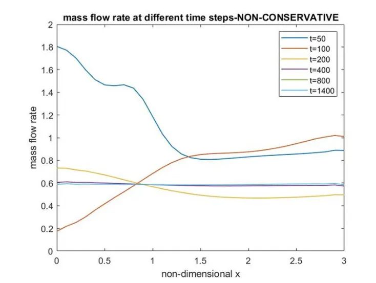
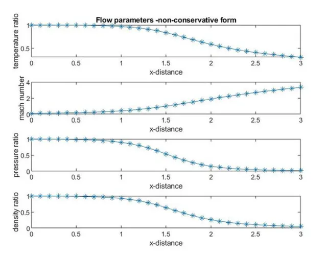
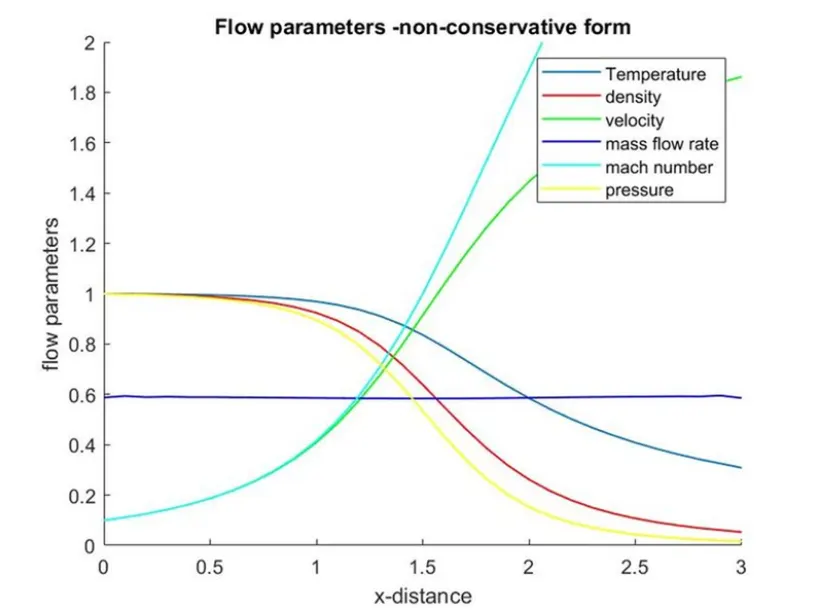
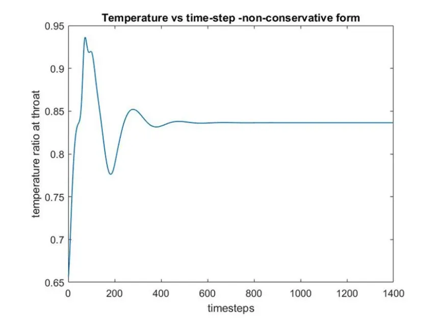
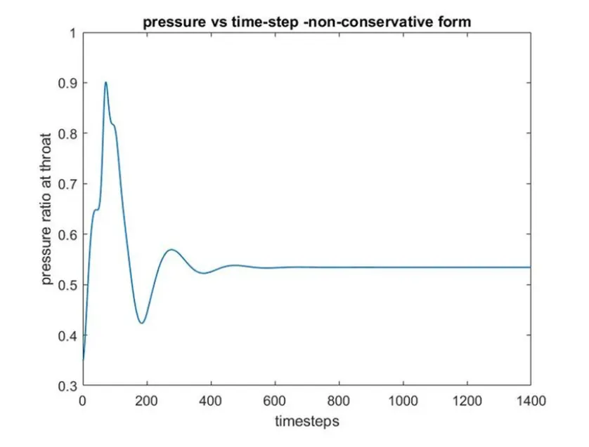
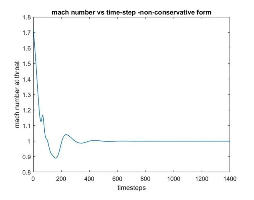
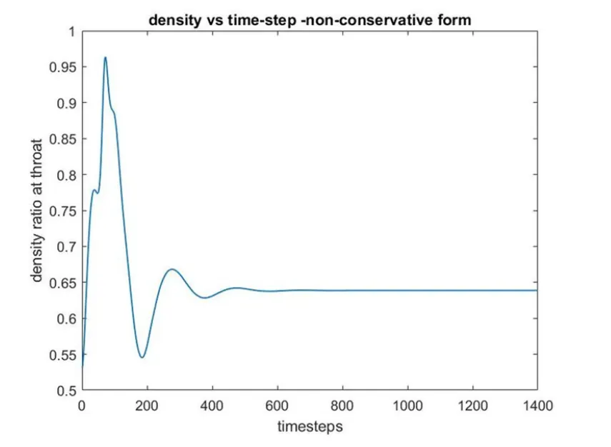
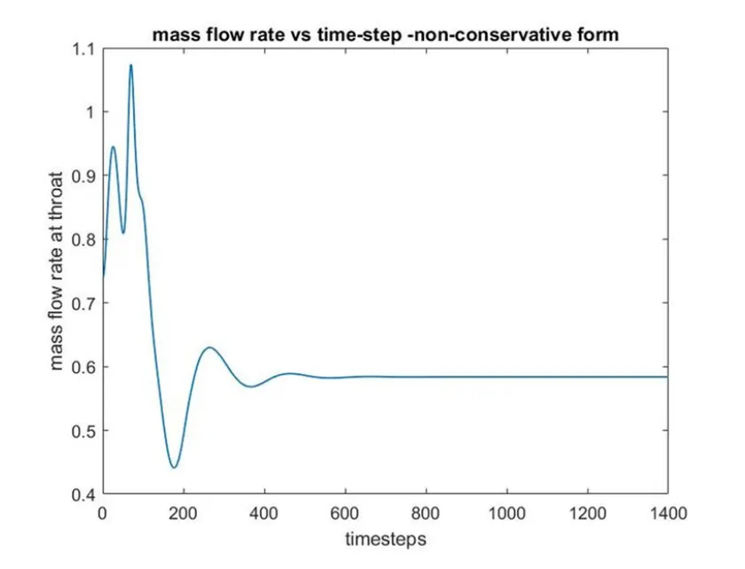
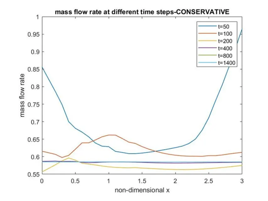
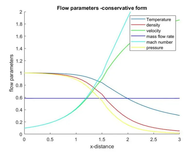
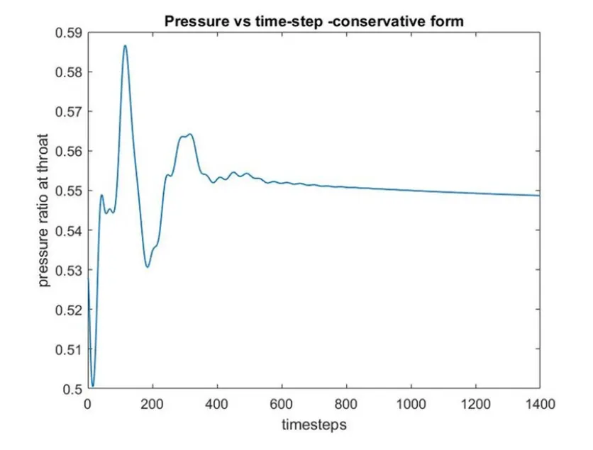
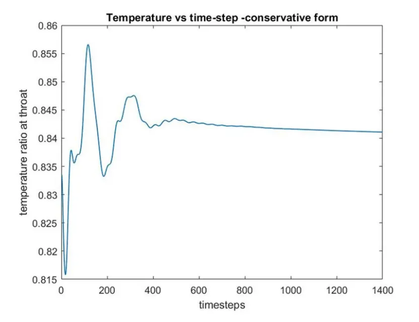
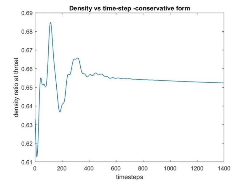
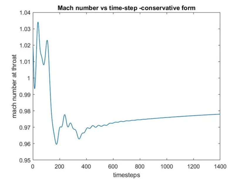
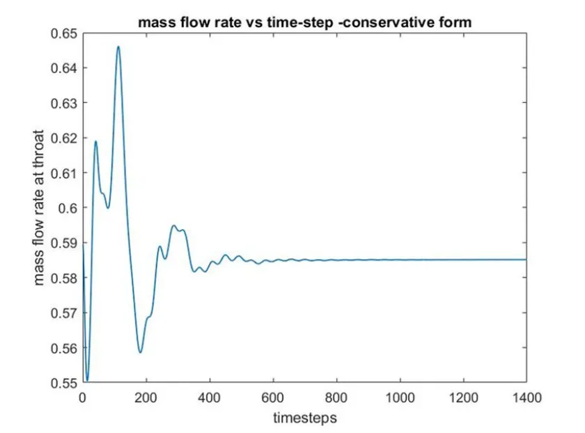
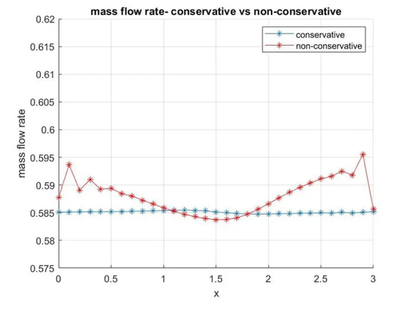
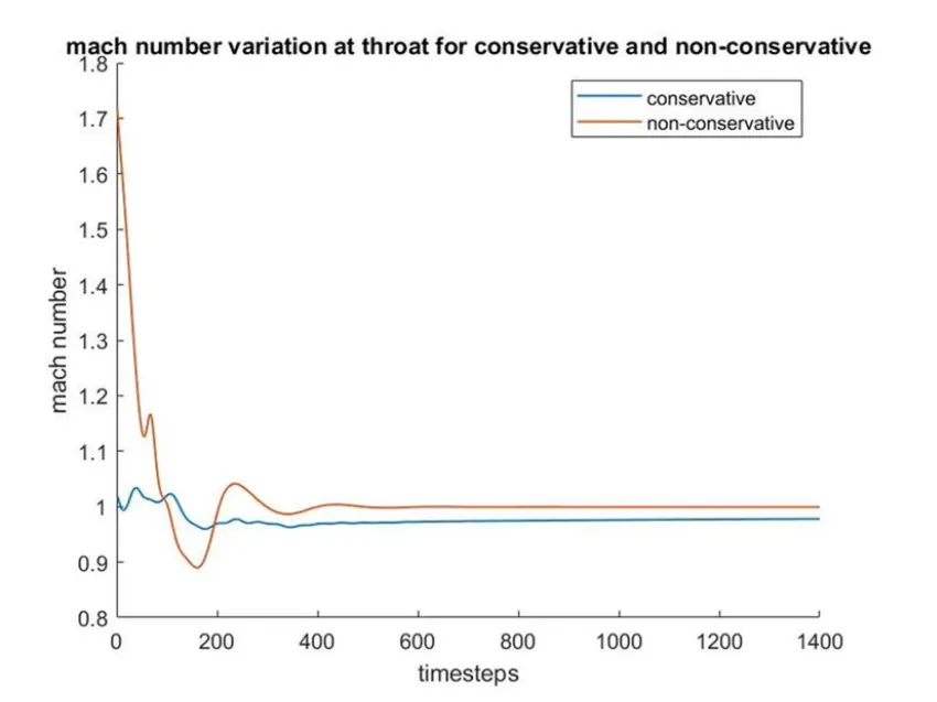
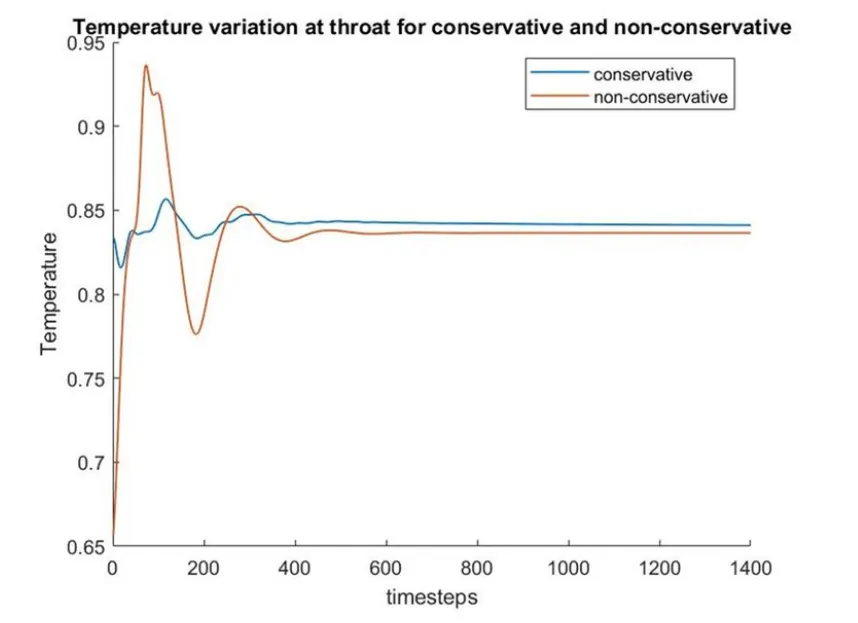
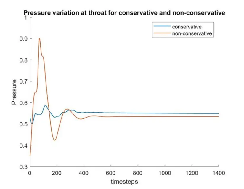
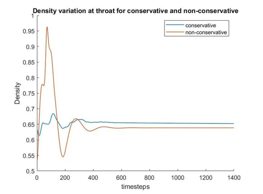
The flow parameters (non dimensional) at the throat are compared
| n | density | pressure | temperature | mach number | |
| conservative |
31 61 |
0.6524 0.6390 |
0.5487 0.5340 |
0.8411 0.8357 |
0.9780 0.9978 |
| non conservative |
31 61 |
0.6387 0.6377 |
0.5342 0.5327 |
0.8365 0.8354 |
0.9994 0.9998 |
CFL Number dependency test
| CFL | density | pressure | temperature | mach number | |
|
Conservative |
0.5 0.8 1 1.2 |
0.6524 0.6461 0.6437 0.6426 |
0.5487 0.5413 0.5385 0.5371 |
0.8411 0.8378 0.8366 0.8359 |
0.9780 0.9899 0.9942 0.9965 |
| Non Conservative |
0.5 0.8 1 1.2 |
0.6387 0.6393 0.6397 NaN |
0.5342 0.5349 0.5353 NaN |
0.8365 0.8367 0.8368 NaN |
0.9994 0.9991 0.9988 NaN |
Conclusion
- The flow parameters in non conservative form become constant after 600th time step, wheras the same occur in conservative form after 800th time step
- It can be seen from the CFL number test that CFL number doesn't have a significant impact on conservative form, whereas, in non-conservative form, the parametr values increases with cFL number, however, the solution blows-off when it hits 1.2