Week 7 - Simulation of a 1D Supersonic nozzle flow simulation using Macormack Method
Week 7 - Simulation of a 1D Supersonic nozzle flow simulation using Macormack Method
In this challenge you are going to simulate the isentropic flow through a quasi 1D subsonic-supersonic nozzle. You will derive both the conservation and non-conservation forms of the governing equations and sovle them using the MacCormack's technique. You need to determine the steady-state temperature distribution for the flow-field variables and investigate the difference between the two forms of governing equations by comparing their solutions.
You need to show the following plots inside your report
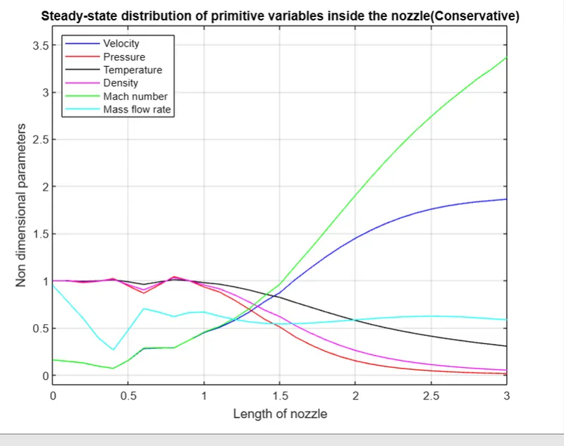
1. Steady-state distribution of primitive variables inside the nozzle
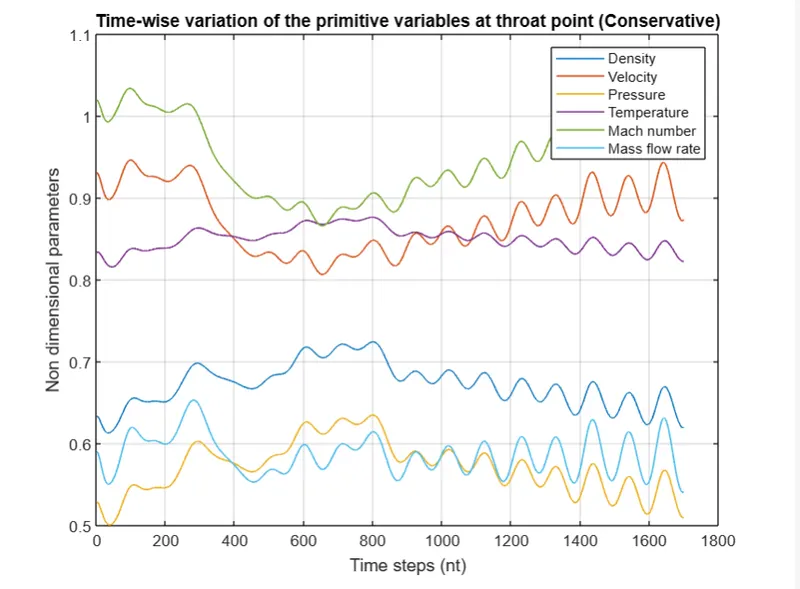
2. Time-wise variation of the primitive variables
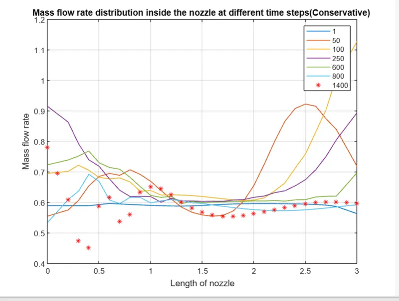
3. Variation of Mass flow rate distribution inside the nozzle at different time steps during the time-marching process
4. Comparison of Normalized mass flow rate distributions of both forms
Expected Results:
- Perform a grid independence test on the solution and expain all your findings.
- The code must be modular. You need to write separate functions to solve both forms.
- Discuss all the plots you are providing with observed inferences.
THEORY:
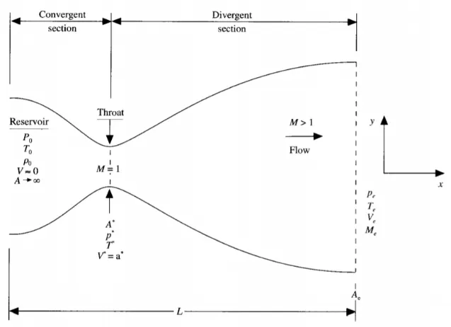
Consider Isentropic flow through a convergent-divergent nozzle. The flow at the inlet of the nozzle comes from the reservoir. The cross-section area of the reservoir is very large and hence velocity is very small(i.e v = 0 m/s at the inlet). The flow is locally subsonic in the convergent section of the nozzle, Sonic at the throat, and Supersonic at the divergent section. The 1D convergent-divergent nozzle is shown below,
Let us consider a small control volume near the throat of the nozzle as shown below,
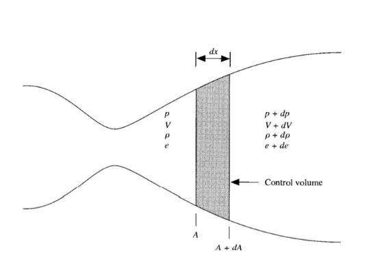
Assume that at a given section, the cross-section area is A, and the flow properties are uniform across the section. Hence, although the area of the nozzle changes as a function of distance along the nozzle, X, and therefore in reality the flow field is two-dimensional (the flow varies in the two-dimensional x-y space), We make the assumption that the flow properties vary only with X; this is tantamount to assuming uniform flow properties across any given cross-section. Such flow is defined as a Quasi-one-dimensional flow.
Governing Equations are represented in terms of PDE for both forms in order to use the Time Marching solution for the problem. The continuity, momentum, and energy governing equations (in terms of non-dimensional variables) for this quasi-one-dimensional steady isentropic flow can be expressed respectively as:
Non- Conservative Form:
1) Continuity equation,

2) Momentum equation,

3) Energy equation,

Conservative Form:
1) Continuity equation,
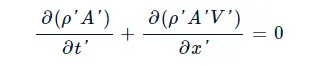
2) Momentum equation,

3) Energy equation,

Maccormack method:
In this method, we split Time Marching into Predictor and corrector phases.
i) Initial Conditions -The initial conditions of the profile for all the flow field variables which are velocity, density, and temperature have to be determined. These are guess values but should be specified with more awareness of the problem.
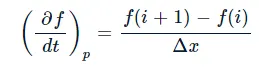
ii) Predictor Step - In this step, perform forward differencing for the space terms,
iii) Solution Update - with the predictor values, the initial solutions are updated,
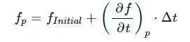
iv) Corrector Step - In this step, perform backward differencing for the space terms,
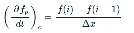
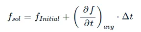
v) Average Derivative - find the average for predictor and corrector steps,

vi) Final solution update - Final solution of the flow field variables for the first time step,
MATLAB CODE :
MAIN CODE & FUNCTION CODE :
close all
clear all
clc

% Length of nozzle
L = 3;
% Grid points
n = [31 71];
% Time steps
nt = 1:1700; % Reduced the number of time steps for simplicity
% CFL number
cfl = 0.2; % Changed CFL number for experimentation

for i = 1:length(n)
    x = linspace(0, L, n(i));

    % Call non-conservative and conservative functions
    [mfr_nc, mfr_throat_nc] = non_conservative(L, n(i), nt, cfl);
    [mfr_c, mfr_throat_c] = conservative(L, n(i), nt, cfl);

    % Plotting
    figure(1)
    subplot(2, 1, 1)
    plot(nt, mfr_throat_c, 'b', nt, mfr_throat_nc, 'r', 'linewidth', 1)
    xlabel('Time steps (nt)')
    ylabel('Mass flow rate')
    legend('Conservative form', 'Non-Conservative form')
    title('Mass flow rate at throat point')
    grid on
    figure(7)
subplot(2,1,1)
plot(nt,mfr_throat_c,'b',nt,mfr_throat_nc,'r','linewidth',1)
xlabel('Time steps (nt)')
ylabel('Mass flow rate')
legend('Conservative form','Non-Conservative form')
title('Mass flow rate"(Non-Conservative vs Conservative)" at throat point ')
grid on
subplot (2,1,2)
plot(x,mfr_c,'b',x,mfr_nc,'r','linewidth',1)
xlabel('Length of nozzle')
ylabel('Mass flow rate')
legend('Conservative form','Non-Conservative form')
title('Mass flow rate"(Non-Conservative vs Conservative)" in the nozzle')
grid on

figure(8)
subplot (2,1,1)
plot(nt,mfr_throat_c,'linewidth',1)
hold on
xlabel('Time steps (nt)')
ylabel('Mass flow rate')
legend('31st node','61st node')
title('Grid independency test at throat point(Conservative)')
grid on
subplot (2,1,2)
plot(nt,mfr_throat_nc,'linewidth',1)
hold on
xlabel('Time steps (nt)')
ylabel('Mass flow rate')
legend('31st node','61st node')
title('Grid independency test at throat point(Non-Conservative)')
grid on

figure(9)
subplot (2,1,1)
plot(x,mfr_c,'linewidth',1)
hold on
xlabel('Length of nozzle')
ylabel('Mass flow rate')
legend('31st node','61st node')
title('Grid independency test at the nozzle(Conservative form)')
grid on
subplot (2,1,2)
plot(x,mfr_nc,'linewidth',1)
hold on
xlabel('Length of nozzle')
ylabel('Mass flow rate')
legend('31st node','61st node')
title('Grid independency test at the nozzle(Non-Conservative form)')
grid on

end


 %FUNCTION CODE FOR NON CONSERVATIVE FORM

function [mfr_nc,mfr_throat_nc]=non_conservative(L,n,nt,cfl)


x=linspace(0,L,n);
dx=x(2)-x(1);

% initial conditions rho, a, v, T, mfr, M, p
rho = 1-0.3146*x;
T= 1-0.2314*x;
v=(0.1+1.09*x).*T.^0.5;
%area
a= 1+2.2*(x-1.5).^2;
M= v./(T.^0.5);
mfr = rho.*a.*v;
p=rho.*T;
g = 1.4;%gamma value

for z=1:31
    u=(T(z))^(1/2);
    dt(z) = cfl*dx/(u + v(z));
end
dt=min(dt);

for i = 1:length(nt)
  %storing initial values
    rho_old = rho;
    T_old = T;
    v_old = v;
  for j=2:n-1
  %predictor step
    drho_dx = (rho(j+1)-rho(j))/dx;
    dv_dx = (v(j+1)-v(j))/dx;
    dT_dx = (T(j+1)-T(j))/dx;
    da_dx = (log(a(j+1))-log(a(j)))/dx;
     % continuity equation
    drho_dt_p(j) = -rho(j)*dv_dx - rho(j)*v(j)*da_dx - v(j)*drho_dx;
    % momentum equation
    dv_dt_p(j) = -v(j)*dv_dx - (1/g)*(dT_dx + (T(j)/rho(j))*drho_dx);
     % energy equation
    dT_dt_p(j) = -v(j)*dT_dx - (g-1)*T(j)*(dv_dx + v(j)*da_dx);
     %updating primitives
    v(j) = v_old(j) + dv_dt_p(j)*dt;
    rho(j) = rho_old(j) + drho_dt_p(j)*dt;
    T(j) = T_old(j) + dT_dt_p(j)*dt;
  %corrector step
    drho_dx = (rho(j)-rho(j-1))/dx;
    dv_dx = (v(j)-v(j-1))/dx;
    dT_dx = (T(j)-T(j-1))/dx;
    da_dx = (log(a(j))-log(a(j-1)))/dx;
     % continuity equation
    drho_dt_c(j) = -rho(j)*dv_dx - rho(j)*v(j)*da_dx - v(j)*drho_dx;
    % momentum equation
    dv_dt_c(j) = -v(j)*dv_dx - (1/g)*(dT_dx + (T(j)/rho(j))*drho_dx);
    % energy equation
    dT_dt_c(j) = -v(j)*dT_dx - (g-1)*T(j)*(dv_dx + v(j)*da_dx);
  end
  %average time derivatives
    drho_dt_avg = 0.5*(drho_dt_p + drho_dt_c);
    dv_dt_avg = 0.5*(dv_dt_p + dv_dt_c);
    dT_dt_avg = 0.5*(dT_dt_p + dT_dt_c);
  %final corected values
  for k = 2:n-1
    rho(k) = rho_old(k) + drho_dt_avg(k)*dt;
    v(k) = v_old(k) + dv_dt_avg(k)*dt;
    T(k) = T_old(k) + dT_dt_avg(k)*dt;
  end
  %entry boundary conditions
    v(1) = 2*v(2)-v(3);
  %exit boundary conditions
    v(n) = 2*v(n-1)-v(n-2);
    rho(n) = 2*rho(n-1)-rho(n-2);
    T(n) = 2*T(n-1)-T(n-2);
  %Final update of primitives
    p = rho.*T;
    M= v./T.^0.5;
    error(k) =  abs(v(k)-v(k-1));
    mfr= rho.*a.*v;
  %to find values at throat point
    T_throat(i) = T(16);
    rho_throat(i) = rho(16);
    v_throat(i) = v(16);
    M_throat(i) = M(16);
    p_throat(i) = p(16);
    error_throat(i)=error(16);
    mfr_throat(i)=mfr(16);
    if n==31
for ii=[1:50:201 700]
    if ii==i
       figure(1)
     plot(x,mfr,'linewidth',1)
     hold on
     title ('Mass flow rate inside the nozzle at different time steps(Non-Conservative)')
     xlabel('Length of nozzle')
     ylabel('Mass flow rate')
    elseif i==1400
     plot(x,mfr,'*r')
     legend('1','50','100','250','600','800','1400')
     grid on
    end
end
end

end
if n==31
figure(2)
     plot(x,v,'b',x,p,'r',x,T,'k',x,rho,'m',x,M,'g',x,mfr,'c')
     ylim([-0.1 3.7])
     title (sprintf('Time step = %d',i))
     xlabel('Length of nozzle')
     ylabel('Non dimensional parameters')
     legend('Velocity','Pressure','Temperature','Density','Mach number','Mass flow rate','location','northwest')
     title('Steady-state distribution of primitive variables inside the nozzle(Non-Conservative)')
     grid on

figure (3)
plot(nt,rho_throat)
hold on
plot(nt,v_throat,'linewidth',1)
plot(nt,p_throat,'linewidth',1)
plot(nt,T_throat,'linewidth',1)
plot(nt,M_throat,'linewidth',1)
plot(nt,mfr_throat,'linewidth',1)
xlabel('Time steps (nt)')
ylabel('Non dimensional parameters')
legend('Density','Velocity','Pressure','Temperature','Mach number','Mass flow rate')
title('Time-wise variation of the primitive variables at throat point(Non-Conservative)')
grid on
end
mfr_nc=mfr;
mfr_throat_nc=mfr_throat;
end
%FUNCTION CODE FOR CONSERVATIVE FORM

function [mfr_c,mfr_throat_c]=conservative(L,n,nt,cfl)

x=linspace(0,L,n);
dx=x(2)-x(1);

% initial conditions rho, a, v, T, M, mfr, p
for ii=1:length(x)
    if (x(ii)<=0.5)
        rho(ii) = 1;
        T(ii) = 1;
    elseif (x(ii)>0.5) & (x(ii)<=1.5)
        rho(ii) = 1-0.366*(x(ii)-0.5);
        T(ii)= 1-0.167*(x(ii)-0.5);
    elseif (x(ii)>1.5) & (x(ii)<=3.5)
        rho(ii) = 0.634-0.3879*(x(ii)-1.5);
        T(ii)= 0.833-0.3507*(x(ii)-1.5);
    end
end
a= 1+2.2*(x-1.5).^2;     %area
g = 1.4;                 %gamma value
% solution vectors u1, u2, u3
u1 = rho.*a;
u2 = 0.59*ones(1,n);
v=u2./u1;
u3 = u1.*((T./(g-1))+(g/2).*v.^2);

M= v./(T.^0.5);
mfr = rho.*a.*v;         %mass flow rate
p=rho.*T;                %pressure


for z=1:31
u=(T(z))^(1/2);
dt(z) = cfl*dx/(u + v(z));
end
dt=min(dt);

for i = 1:length(nt)
    %storing initial values
    u1_old = u1;
    u2_old = u2;
    u3_old = u3;

    for j=2:n-1
   %flux vectors
        f1 = u2;
        f2 = ((u2.^2)./u1)+((g-1)/g)*(u3-((g/2)*(u2.^2)./u1));
        f3 = ((g.*u2.*u3)./u1) - ((g*(g-1)/2)*(u2.^3)./(u1.^2));
   %source term
        j1 = (1/g)*rho(j)*T(j)*((a(j+1)-a(j))/dx);
   %predictor step
   %continuity equation
        du1_dt_p(j)= -(f1(j+1)-f1(j))/dx;
   %momentum equation
        du2_dt_p(j)= -(f2(j+1)-f2(j))/dx + j1;
   %energy equation
        du3_dt_p(j)= -(f3(j+1)-f3(j))/dx;
   %updating solution vectors
        u1(j) = u1_old(j) + du1_dt_p(j)*dt;
        u2(j) = u2_old(j) + du2_dt_p(j)*dt;
        u3(j) = u3_old(j) + du3_dt_p(j)*dt;
   %updating primitives
        rho=u1./a;
        T=(g-1).*(u3./u1-(g/2).*(u2./u1).^2);
   %updating flux terms
        f1=u2;
        f2=u2.^2./u1+((g-1)/g).*(u3-(g/2)*u2.^2./u1);
        f3=g.*u2.*u3./u1-0.5*g*(g-1).*u2.^3./u1.^2;
   %source term for corrector step
        j2 = (1/g)*(rho(j)*T(j)*(a(j)-a(j-1))/dx);
   %corrector step
   %continuity equation
        du1_dt_c(j) = -(f1(j)-f1(j-1))/dx;
   %momentum equation
        du2_dt_c(j) = -(f2(j)-f2(j-1))/dx + j2;
   %energy equation
        du3_dt_c(j) = -(f3(j)-f3(j-1))/dx;
    end
    %average time derivatives
        du1_dt_avg = 0.5*(du1_dt_p + du1_dt_c);
        du2_dt_avg = 0.5*(du2_dt_p + du2_dt_c);
        du3_dt_avg = 0.5*(du3_dt_p + du3_dt_c);
    %final corected values
    for k = 2:n-1
        u1(k) = u1_old(k) + du1_dt_avg(k)*dt;
        u2(k) = u2_old(k) + du2_dt_avg(k)*dt;
        u3(k) = u3_old(k) + du3_dt_avg(k)*dt;
    end
    %entry boundary conditions
        u1(1) = a(1);
        u2(1) = 2*u2(2)-u2(3);
        u3(1) = u1(1)*(T(1)/(g-1) + (g*(u2(1)/u1(1))^2)/2);
    %exit boundary conditions
        u1(n) = 2*u1(n-1)-u1(n-2);
        u2(n) = 2*u2(n-1)-u2(n-2);
        u3(n) = 2*u3(n-1)-u3(n-2);

    %Final update of primitives
        rho = u1./a;
        v = u2./u1;
        T=(g-1).*(u3./u1-(g/2).*(u2./u1).^2);
        p = rho.*T;
        M= v./T.^0.5;
        error(k) =  abs(v(k)-v(k-1));
        mfr= u2;
  %to find values at throat point
    T_throat(i) = T(16);
    rho_throat(i) = rho(16);
    v_throat(i) = v(16);
    M_throat(i) = M(16);
    p_throat(i) = p(16);
    error_throat(i)=error(16);
    mfr_throat(i)=mfr(16);

if n==31
    for ii=[1:50:201 700]
    if ii==i
       figure(4)
     plot(x,mfr,'linewidth',1)
     hold on
     title ('Mass flow rate distribution inside the nozzle at different time steps(Conservative) ')
     xlabel('Length of nozzle')
     ylabel('Mass flow rate')
    elseif i==1400
     plot(x,mfr,'*r')
     legend('1','50','100','250','600','800','1400')
     grid on
    end
end
end

end
if n==31
figure(5)
     plot(x,v,'b',x,p,'r',x,T,'k',x,rho,'m',x,M,'g',x,mfr,'c')
     ylim([-0.1 3.7])
     title (sprintf('Time step = %d',i))
     xlabel('Length of nozzle')
     ylabel('Non dimensional parameters')
     legend('Velocity','Pressure','Temperature','Density','Mach number','Mass flow rate','location','northwest')
     title('Steady-state distribution of primitive variables inside the nozzle(Conservative)')
     grid on

figure (6)
plot(nt,rho_throat)
hold on
plot(nt,v_throat,'linewidth',1)
plot(nt,p_throat,'linewidth',1)
plot(nt,T_throat,'linewidth',1)
plot(nt,M_throat,'linewidth',1)
plot(nt,mfr_throat,'linewidth',1)
xlabel('Time steps (nt)')
ylabel('Non dimensional parameters')
legend('Density','Velocity','Pressure','Temperature','Mach number','Mass flow rate')
title('Time-wise variation of the primitive variables at throat point (Conservative)')
grid on
end
mfr_c=mfr;
mfr_throat_c=mfr_throat;

end
Main Code Explanation: The main code starts by clearing any existing data and setting up the initial parameters for the simulation. The key parameters defined are:
L: Length of the nozzle.n: An array specifying the number of grid points to use for the simulation. Two different grid sizes are considered.nt: An array representing the time steps for which the simulation will run.cfl: The Courant-Friedrichs-Lewy (CFL) number, which is a stability criterion for time-stepping methods in fluid dynamics.
The main part of the code then iterates through each grid size defined in the n array. For each grid size, it does the following:
- Generates the grid points along the length of the nozzle (
x). - Calls the function
non_conservativeandconservativefor both non-conservative and conservative forms, respectively, passing the relevant parameters. - Plots various results comparing the non-conservative and conservative forms, grid independence tests, and more using MATLAB's plotting functions.
Function Code for Non-Conservative Form (non_conservative): This function code defines the behavior of the simulation using the non-conservative form of the governing equations. The key steps in this function are:
- Initializing the initial conditions for density (
rho), temperature (T), velocity (v), area (a), and other variables. - Calculating the time step (
dt) for each grid point based on the CFL condition. - Iterating over the time steps (
nt) to simulate the flow dynamics.- Predictor step: Calculates derivatives and updates variables for continuity, momentum, and energy equations.
- Corrector step: Calculates derivatives again based on updated values and updates variables.
- Applies boundary conditions at entry and exit points of the nozzle.
- Computes derived variables like pressure (
p), Mach number (M), and mass flow rate (mfr). - Stores values at the throat point (16th node) for each time step.
- Generates plots at specific time steps for mass flow rate distribution and steady-state distribution of primitive variables.
Function Code for Conservative Form (conservative): This function code defines the behavior of the simulation using the conservative form of the governing equations. The key steps in this function are:
- Initializing the initial conditions for density (
rho), temperature (T), velocity (v), and other variables. - Calculating the time step (
dt) for each grid point based on the CFL condition. - Iterating over the time steps (
nt) to simulate the flow dynamics.- Calculates flux vectors and source terms.
- Predictor step: Updates solution vectors for continuity, momentum, and energy equations.
- Corrector step: Updates solution vectors based on averaged derivatives.
- Applies boundary conditions at entry and exit points of the nozzle.
- Computes derived variables like pressure (
p), Mach number (M), and mass flow rate (mfr). - Stores values at the throat point (16th node) for each time step.
- Generates plots at specific time steps for mass flow rate distribution and steady-state distribution of primitive variables.
Both function codes update the primitive variables like density, velocity, and temperature based on their respective forms of governing equations and utilize predictor-corrector numerical methods to advance in time. The main difference between the two lies in the formulation of these equations and the corresponding flux and source terms used for the updates.
PLOT EXPLANATION :
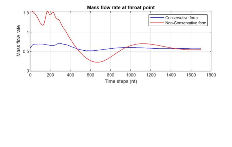
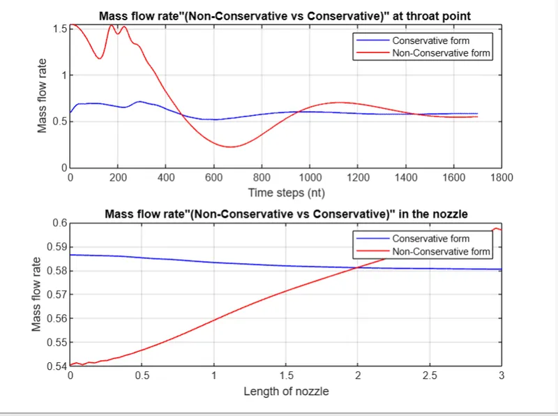
Mass Flow Rate at Throat Point (Non-Conservative vs Conservative):
- This plot compares the mass flow rate at the throat point (31st node) over the specified number of time steps.
- The x-axis represents time steps (nt), and the y-axis represents the mass flow rate.
- Two lines are plotted: one for the conservative form and one for the non-conservative form.
- The legend indicates which line corresponds to which form.
- The title of the plot is "Mass flow rate at throat point."
Mass Flow Rate Comparison (Non-Conservative vs Conservative):
- This plot has two subplots. The first subplot displays the mass flow rate at the throat point (31st node) for both the conservative and non-conservative forms.
- The second subplot displays the mass flow rate profiles along the length of the nozzle for both forms.
- The x-axis of the first subplot represents time steps (nt), and the y-axis represents the mass flow rate.
- The x-axis of the second subplot represents the length of the nozzle, and the y-axis represents the mass flow rate.
- Legends indicate the corresponding form for each line.
- The title of the first subplot is "Mass flow rate (Non-Conservative vs Conservative) at throat point."
- The title of the second subplot is "Mass flow rate (Non-Conservative vs Conservative) in the nozzle."
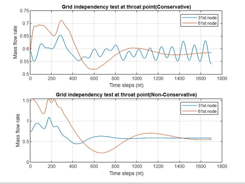
Grid Independence Test at Throat Point (Conservative):
- This plot compares the mass flow rate at the throat point (31st and 61st nodes) using the conservative form.
- Two lines are plotted, each corresponding to different grid nodes.
- The x-axis represents time steps (nt), and the y-axis represents the mass flow rate.
- The legend indicates which line corresponds to which grid node.
- The title of the plot is "Grid independence test at throat point (Conservative)."
Grid Independence Test at Throat Point (Non-Conservative):
- This plot is similar to the previous plot but uses the non-conservative form.
- It compares the mass flow rate at the throat point (31st and 61st nodes) using the non-conservative form.
- The x-axis represents time steps (nt), and the y-axis represents the mass flow rate.
- The legend indicates which line corresponds to which grid node.
- The title of the plot is "Grid independence test at throat point (Non-Conservative)."
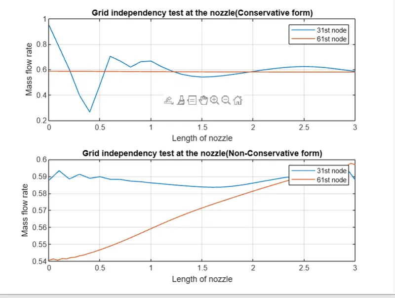
Grid Independence Test in the Nozzle (Conservative):
- This plot compares the mass flow rate along the length of the nozzle (31st and 61st nodes) using the conservative form.
- Two lines are plotted, each corresponding to different grid nodes.
- The x-axis represents the length of the nozzle, and the y-axis represents the mass flow rate.
- The legend indicates which line corresponds to which grid node.
- The title of the plot is "Grid independence test in the nozzle (Conservative)."
Grid Independence Test in the Nozzle (Non-Conservative):
- This plot is similar to the previous plot but uses the non-conservative form.
- It compares the mass flow rate along the length of the nozzle (31st and 61st nodes) using the non-conservative form.
- The x-axis represents the length of the nozzle, and the y-axis represents the mass flow rate.
- The legend indicates which line corresponds to which grid node.
- The title of the plot is "Grid independence test in the nozzle (Non-Conservative)."
Mass Flow Rate Inside the Nozzle at Different Time Steps (Non-Conservative):
- This plot shows the distribution of mass flow rate along the length of the nozzle at different time steps for the non-conservative form.
- Multiple lines are plotted, each corresponding to a different time step.
- The legend indicates the time step associated with each line.
- The title of the plot is "Mass flow rate distribution inside the nozzle at different time steps (Non-Conservative)."
Steady-State Distribution of Primitive Variables Inside the Nozzle (Non-Conservative):
- This plot displays the steady-state distribution of various primitive variables (velocity, pressure, temperature, density, Mach number, and mass flow rate) inside the nozzle using the non-conservative form.
- Each variable is plotted against the length of the nozzle.
- The legend indicates which variable corresponds to which line.
- The title of the plot indicates the current time step.
Time-Wise Variation of Primitive Variables at Throat Point (Non-Conservative):
- This plot shows the time-wise variation of primitive variables (density, velocity, pressure, temperature, Mach number, and mass flow rate) at the throat point using the non-conservative form.
- Each variable is plotted against time steps (nt).
- The legend indicates which variable corresponds to which line.
- The title of the plot is "Time-wise variation of the primitive variables at throat point (Non-Conservative)."
CONCLUSION :
- The code investigates a compressible flow through a nozzle using both conservative and non-conservative forms of equations.
- The conservative and non-conservative forms lead to different predictions for mass flow rates, indicating the importance of formulation choice.
- Increasing grid resolution results in more accurate and grid-independent predictions for both mass flow rates and other variables.
- The plots capture the dynamic behavior of primitive variables over time and space, providing insights into the transient and steady-state flow characteristics.