Simulation of the 1-D supersonic nozzle flow simulation using the Mac-Cormack's technique:

Deriving the conservative as well as the non-conservative form of the governing equation for the quasi 1-D flow through a nozzle of length 'L' as follows:

We are going to derive a governing equation for the quasi 1-D steady state super-sonic nozzle:

So for that we are going to start from the integral form of the continuity equation and then reach to the PDE form of the continuity equation which will be our derived equation as follows:

We apply this equation to the shaded control volume shown in fig. 1. This control volume is a slice of the nozzle flow, where the infinitesimal thickness of the slice is dx. On the left side of the control volume, consistent with the quasi 1-D assumption, the density, velocity, pressure, and internal energy, denoted by rho,v,p, and e, respectively, are uniform over the area A. Similarly, on the right side of the control volume, the density,velocity,pressure, and internal energy, denoted by rho+drho, v+dv, p+dp, and e+de, respectively, are uniform over the area A+dA. Applied to the control volume in Fig. 1, the volume integral in eq. 2.19 becomes, in the limit as dx becomes very small,

where A dx is the volume of the control volume in the limit of dx becoming vanishing small. The surface integral in Eq. (2.19) becomes

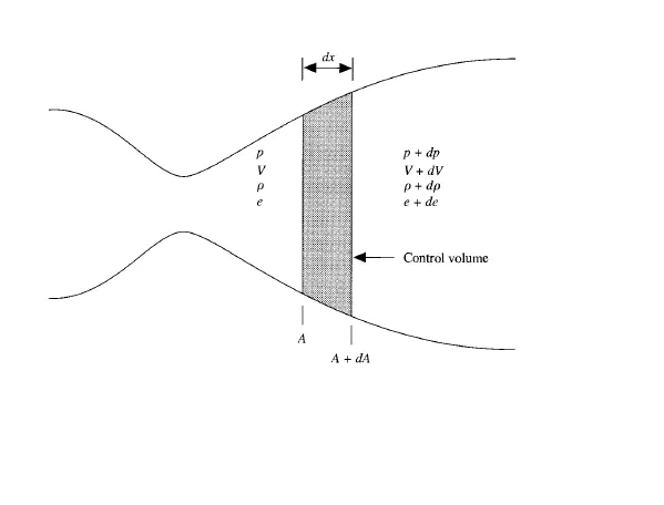
Fig. 1 - Control vol. for deriving the PDE for unsteady,quasi 1-D flow.

where the '-' sign on the leading term on the R.H.S. is due to the vectors v & ds pointing in the opposite directions over the left face of the control volume, & hence the dot product is negative. Expanding the triple product term in eq. 7.11, we have

In the limit as dx becomes very small, the terms involving products of differentials in eq. (7.12), such as rho dv dA, drho dv dA, go to zero much faster than those terms involving only one differential. Hence, in eq. (7.12), all terms involving products of differentials can be dropped, yielding in the limit as dx becomes very small

Substituting Eq.s (7.10) & (7.13) into (2.19), we have

Dividing Eq. (7.14) by dx and noting that d(rho*A*v)/dx is, in the limit as dx goes to zero, the definition of the partial derivative w.r.t. x, we have

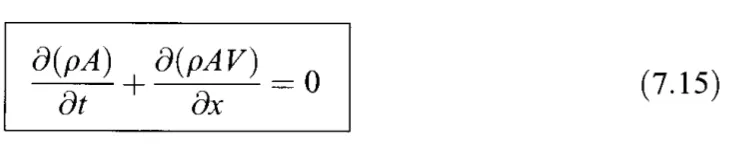
The above eq. is the continuity eq. in the conservation form for quasi 1-D flow.

Non-dimensionalizing the variables of the eq.7, we have

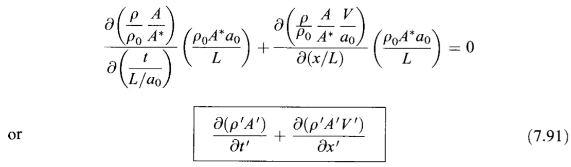
The above eq. is the non-dimensionalized continuity eq. in the conservative form which I have solved in my MATLAB programme using the Mac-Cormack's technique for the simulation of a quasi 1-D flow.

Derivation of the Conservative form of the momentum eq. as follows:

We now turn to the integral form of the x-component of the momentum equation, written below for an inviscid flow (neglecting the viscous stress terms) with no body forces,

where the term (p.ds)_x denotes the x component of the vector p.ds. We apply eq. 8 to the shaded control volume in Fig. 2. In Eq.(8), the integrals on the left side are evaluated in the same manner as discussed above in regard to the continuity equation. That is,

and

The evaluation of the pressure force term on the R.H.S. of Eq.(8) is the best carried out with the aid of Fig.2. Here, the x components of the vector p.ds are shown on all the four sides of the control volume. Remember that ds always points away from the control volume; hence any x component (p.ds) that acts towards the left (in the negative x direction) is a negative quantity, and any x component (p.ds)_x that acts toward the right (in the positive x direction) is a positive quantity. Also note that the x component of p .ds acting on the top and bottom inclined faces of the control volume in Fig.2 can be expressed as the pressure p acting on the component of the inclined area projected perpendicular to the x direction, (dA)/2; hence, the contribution of each inclined face (top or bottom) to the pressure integral in Eq. (8) is -p(dA/2). All together, the R.H.S. of Eq.(8) is expressed as follows:

substituting Eqs. (9) to (11) into (8), we have

Canceling like terms and ignoring products of differentials, Eq.(12) becomes in the limit of dx becoming very small

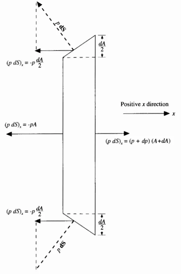
Fig. 7.4: The forces in the x-direction acting on the control volume

Dividing Eq.(13) by dx and taking the limits as dx goes to zero, we obtain the PDE

This is the conservation form of the momentum eq. of the quasi 1-D flow. Let us combine the two x derivatives in eq. 7.23 as follows:

Since

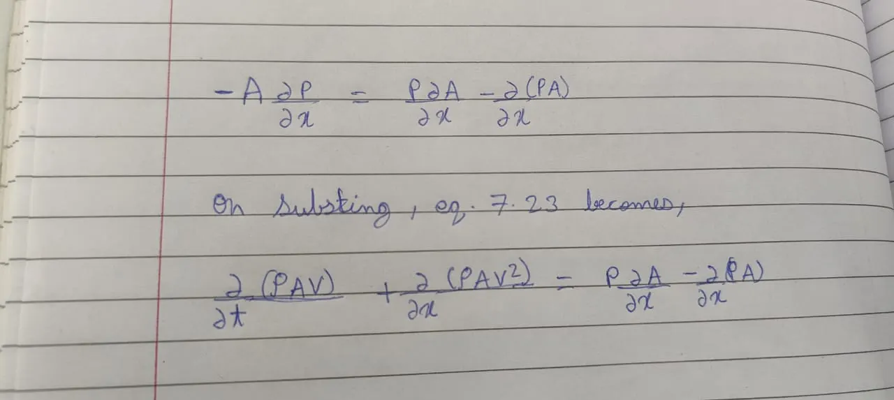
On transposing the second term of R.H.S. in the last eq., we get

Non-dimensionalizing eq. 7.93, we have

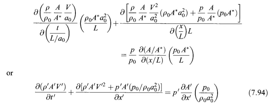
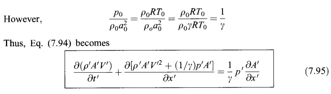
The above eq. is our non-dimensionalized momentum eq. in the conservation form which I have solved in my MATLAB programme using the Mac-Cormack's technique for the simulation of the quasi 1-D flow.

Derivation of the Conservative form of the energy eq. as follows:

Now, let's consider the integral form of the energy equation. For an adiabatic flow(q=0) with no body forces & no viscous effects, the integral form of the energy eq. is

Applied to the shaded control vol. in Fig.1, & keeping in mind the pressure forces shown in Fig.7.4, eq. 7.29 becomes

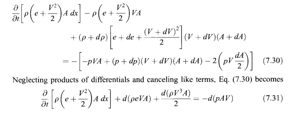
Taking the limits as dx approaches zero, eq.7.32, becomes the following PDE:

Eq. 7.33 is the conservation form of the energy eq. expressed in terms of the total energy e+v^2/2, appropriate for unsteady, quasi 1-D flow.

Combining the x-derivatives in eq. 7.33, we have

Let us define a non-dimensional internal energy as follows:

With this, the non-dimensional form of the eq. 7.96 is obtained as follows:

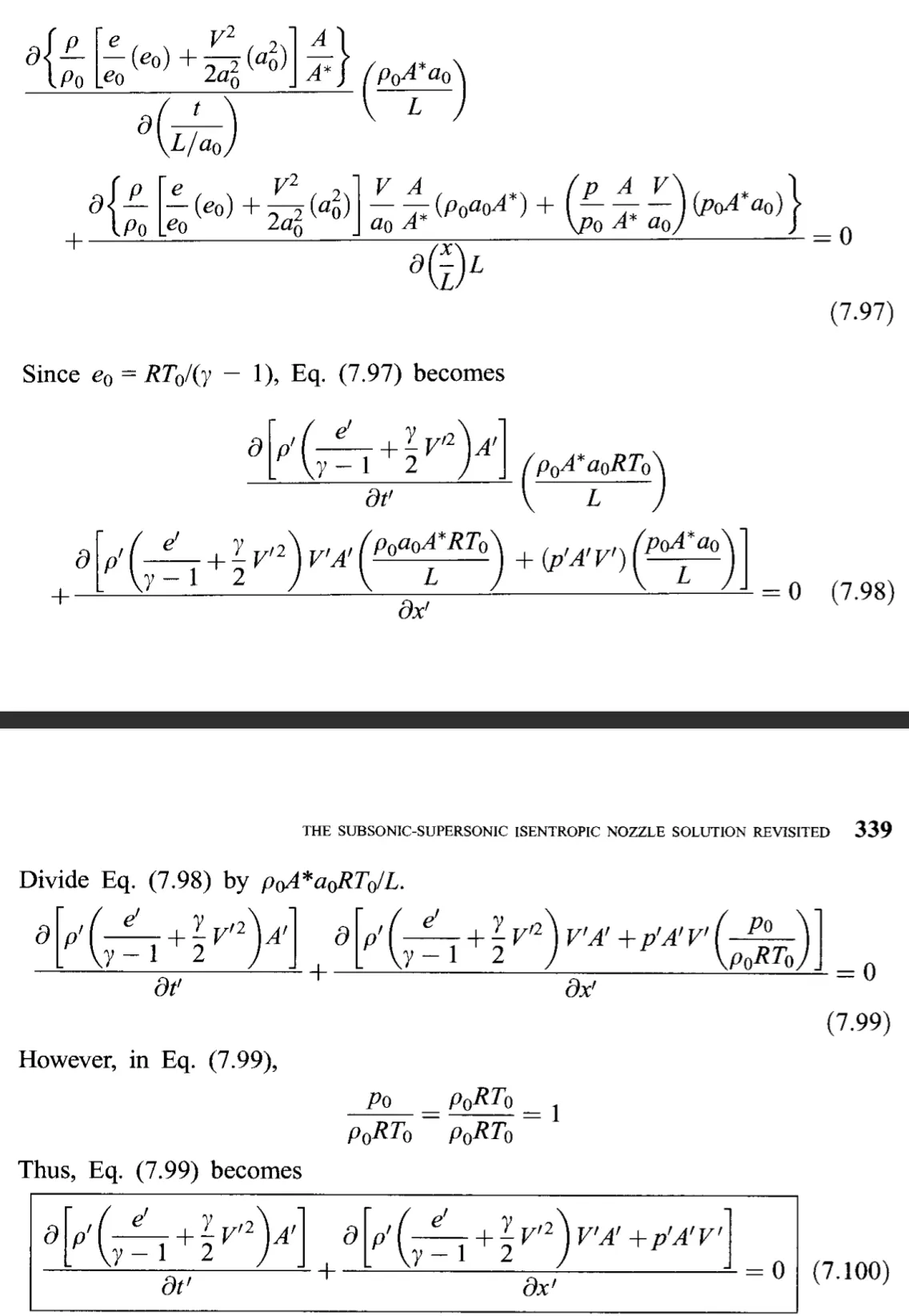
The above eq. is the non-dimensionalized energy eq. in the conservative form which I have solved in my MATLAB programme using the Mac-cormack's technique for the quasi 1-D flow.

Let's have some numerical analysis for the non-dimensionalization of the variables of the quasi 1-D flow:

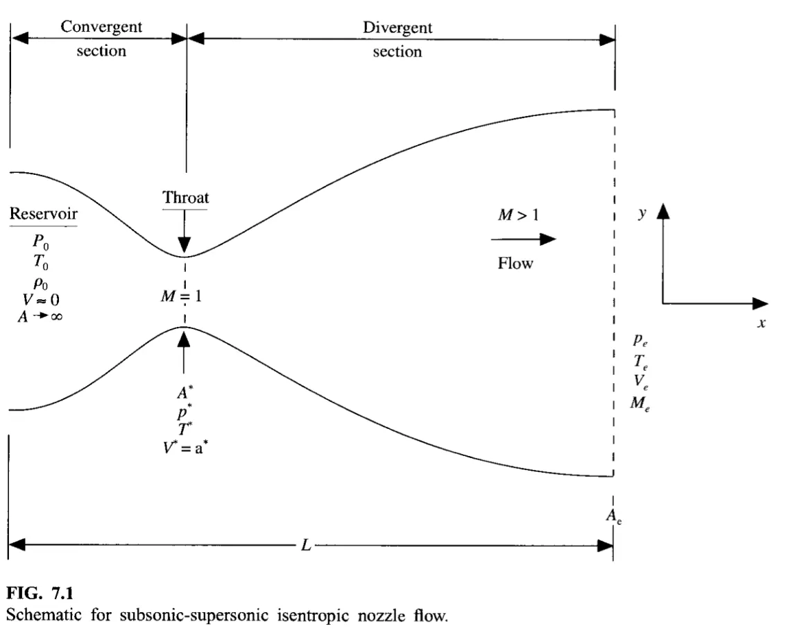
As from the above fig.7.1, where the reservoir temperature & density are denoted by T₀ & respectively, we define the non-dimensional temperature & density, respectively, as

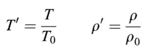
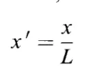
where (for the time being) the prime denotes a dimensionaless variable. Moreover, letting L denote the length of the nozzle, we define a dimensionless length as

Denoting the speed of sound in the reservoir as a₀, where

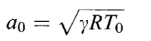
we define a dimensionless velocity as

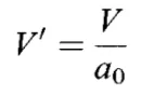
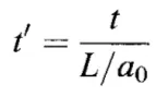
Also, the quantity L/a₀ has the dimension of time, & we define a dimensionless time as

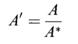
Finally, we ratio the local area A to the sonic throat area A* & define a dimensionless area as

Now, let's move to the derivation of non-conservative form of the governing PDEs of a quasi 1-D subsonic supersonic nozzle as follows:

Derivation of the non-conservative form of the continuity eq. as follows:

Have a look at the continuity eq. 7.15 in conservation form as follows:

On expanding eq.7.15, we have

Introducing the non-dimensional variables to the eq.7.42, we have

Note that A' is a function of x' only; it is not a function of time (the nozzle geometry is fixed, invariant with time). Hence, eq. (7.45) the time derivative can be written as

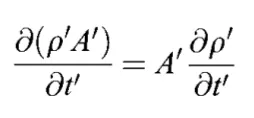
With this, eq. 7.45 becomes

The above eq. is the non-dimensionalized continuity eq. in the non-conservative form which I have solved in my MATLAB programme using the Mac-cormack's technique for the quasi 1-D flow.

Derivation of the non-conservative form of the momentum eq. as follows:

Have a look at the conservation form of the momentum eq. 7.23 as follows:

Have a look at the continuity eq. as 7.15 in conservation form as follows:

Multiplying the above eq. 7.15 by v, we get

& then substracting eq. 7.24 from eq. 7.23, we have

Expanding the derivatives on the L.H.S. of eq. 7.25 & cancelling like terms, we have

Dividing eq. 7.26 by A, then we finally have

This above eq. is the momentum eq. in the non-conservation form for the quasi 1-D flow.

The pressure can be eliminated from the eq. 7.27 by using the eq. of state as:

On differentiating the above eq. 7.40, we have

using the eq. 7.41 in eq. 7.27, we get

Introducing the non-dimensional variables to eq. 7.43, we have

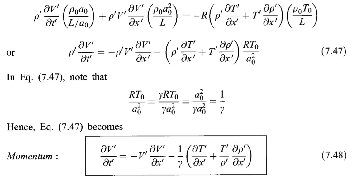
The above eq. is the non-dimensionalized momentum eq. in the non-conservation form which I have solved in my MATLAB programme using the Mac-Cormack's technique for the simulation of the quasi 1-D flow.

Derivation of the non-conservative form of the energy eq. as follows:

Have a look at the conservation form of the energy eq. 7.35 which is expressed in terms of internal energy e as follows:

Now, have a look at the continuity eq. 7.15 which is in the conservation form as follows:

The non-conservation form of the energy eq. is obtained my multiplying the above eq. 7.15 by e,

and substracting eq. 7.36 from eq. 7.35, yielding

Expanding the R.H.S. & dividing by A, eq. 7.37 becomes

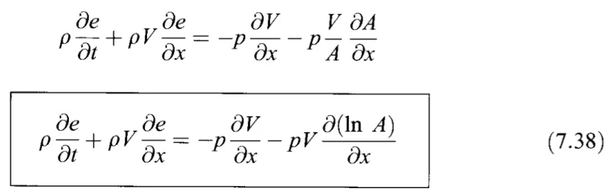
Eq. 7.38 is the non-conservation form of the energy eq. expressed in terms of internal energy, appropraiate to unsteady, quasi 1-D flow.

Since, for a calorically perfect gas

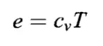
Hence, eq. 7.38 becomes

The pressure can be eliminated from the above eq. by using the eq. of state

on differentiating the above eq. 7.40, we have

With this, we expand the eq. 7.39 as

Introducing the non-dimensional variables to the above eq. 7.44, we have

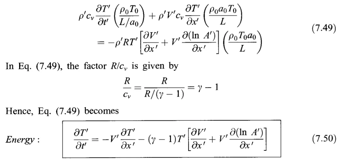
The above eq. 7.50 is the non-dimensionalized energy eq. in the non-conservative form which I have solved in my MATLAB programme using the Mac-Cormack's technique for the simulation of a quasi 1-D flow.

We are going to solve the above derived equations using the Mac-Cormack's technique as follows:

1. Predictor step:

In this step, we discretise the space terms of the PDE into the forward differencing scheme.

After the discretisation, we multiply the result with the time step size 'DT' (adaptive time step) & then add it to its own previous time step value. This step is known to be the solution update as

f^*=f_(initial) + (del(f)/delt)*DT

2. Corrector step:

In this step, we discretise the space terms of the PDE into the backward differencing scheme. In this, we use the update values of the variables which are obtained from the previous step as solution update.

3. Average:

In this step, we average the discretised predictor & corrector step PDE values.

4. Final solution:

The average value is to be multiplied by 'DT' & then this product result is added to the previous time step value of that variable.

Determining the steady-state temperature distribution for the flow field variables using the Mac-Cormack's technique as follows:

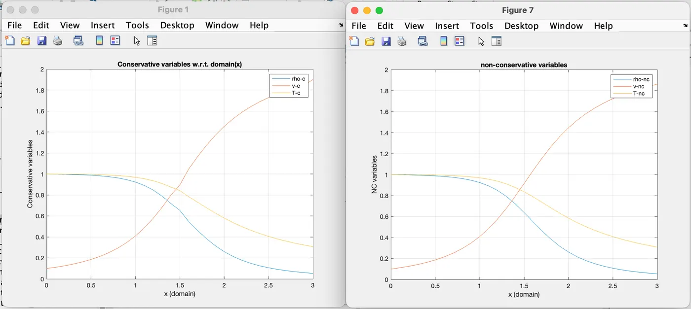
In both the figure windows, the yellow curve is the 'temperature' curve. In the conservative form, the temperature curve deviates a little bit at the throat section as compared to the non-conservative form.

Time-wise variation of the primitive variables as follows:

1. Density(C(conservative) & NC(non-conservative):

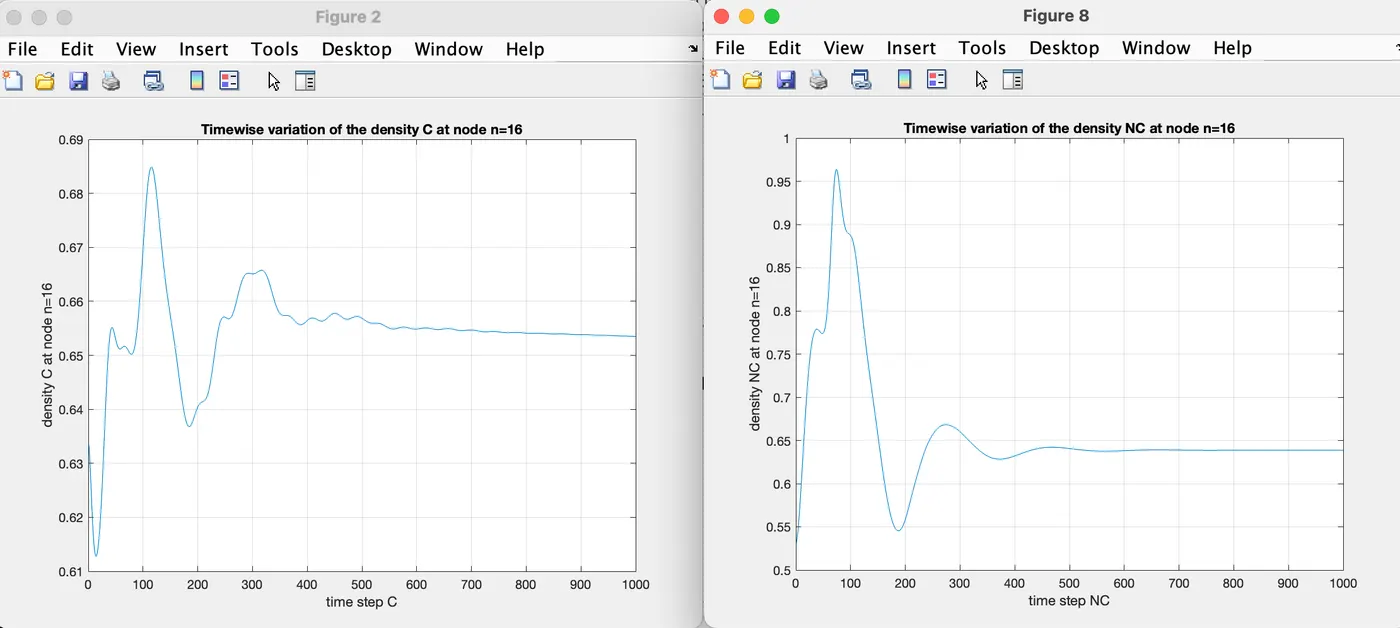
The peak density of the non-conservative form is higher than the conservative form.

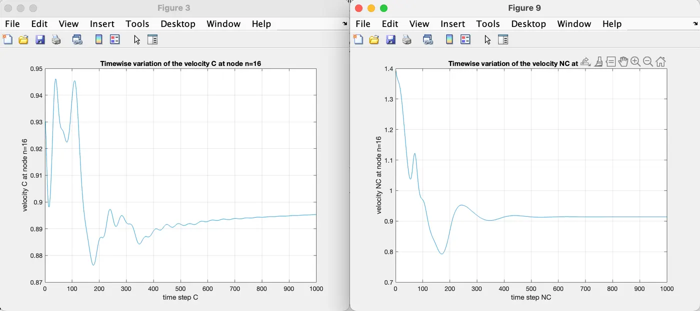
2. Velocity(C(conservative) & NC(non-conservative):

3. Temperature(C(conservative) & NC(non-conservative):

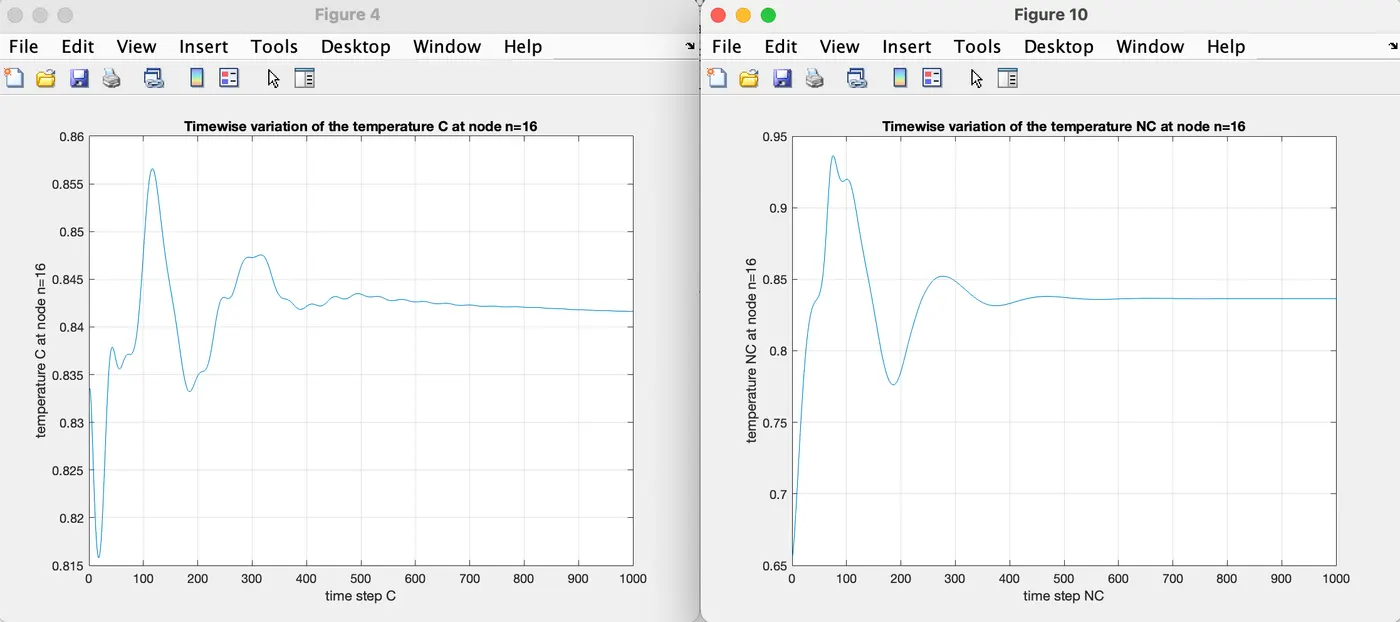
The peak temperature of the non-conservative form is higher than the conservative form.

Variation of the mass-flow rate distribution inside the nozzle at different time steps during the time marching process as follows:

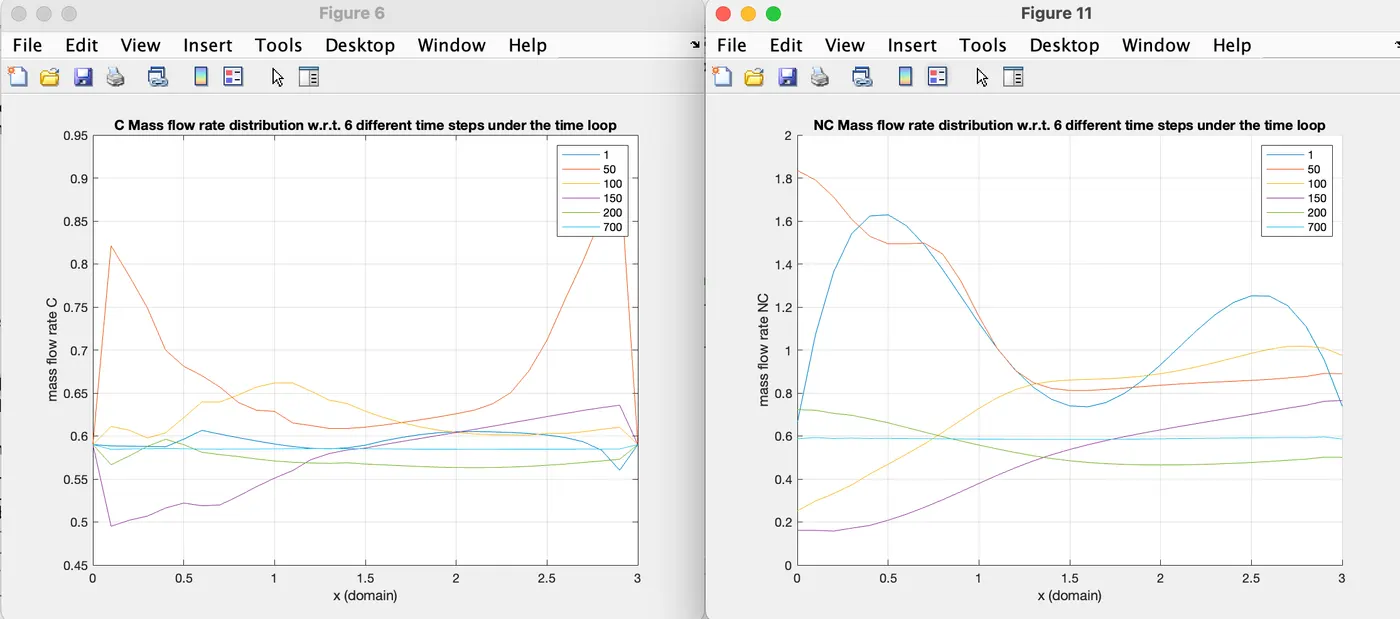
From the observation, it has been observed that the fluctuation in the mass flow rate at specified time steps is higher in case of the non-conservative form as compared to the conservative form.

Comparison of normalised mass flow rate of both the forms:

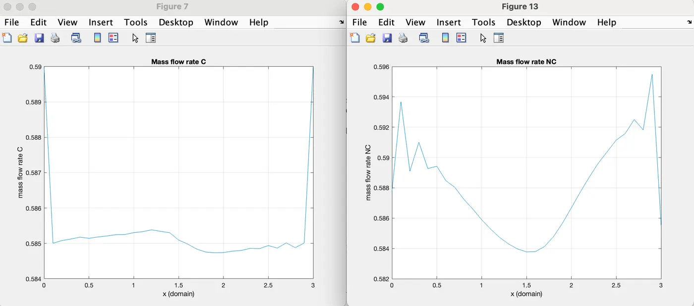
The change in the mass flow rate in the conservative form is not much higher as compared to the mass flow rate in the non-conservative form. So it means that the stability regarding the mass flow rate is higher in the conservative form as compared to the non-conservative form.

Conclusion:

So from the above comparison of the plots between the conservative & the non-conservative, it has been concluded as follows:

1. The rate of steady state is much higher in non-conservative form as compared to the conservative form as we are directly solve for the primitive variables in case of the non-conservative form.
2. The stability in case of shocks is much higher in the conservative form as compared to the non-conservative form because in conservative form, we first solve the flux vector for the solution matrix then we get the primitive variable through the solution matrix. As the change in gradience of the primitive variables are very high so when we directly solve for the primitive variables then we leads to the instability in case of shocks.

So with this, I want to say that I have almost explained everything that has been asked so with that I am going to finish this challenge.