Challenge

Week 4.1 - Genetic Algorithm

KKush Choubisa7 Apr 2022

Aim:- To write a code in MATLAB to optimize the stalagmite function and to find the global maxima of the function.

Objective:- To explain the concept of the used optimization technique is a genetic algorithm that is used in our coding to perform the optimization of the stalagmite function and to find its global maximum.

Concept of optimization:-

Optimization is a decision-making process to obtain the best result. This is used in vast fields to get an optimized result.

The optimization technique follows several methods as can be seen in the following:

Need for optimization
Selecting design variables hello
Formulating design constraints
Formulating function variables
Choosing variable bounds
Choosing optimization algorithm
Best/optimized result

Need for optimization:-

For better understanding let's take an example.

Suppose we want to make a sports car whose design must be aerodynamic to minimize the drag force for a greater velocity. So this car is designed using the concept of fluid mechanics. Using this concept, we may have many designs for the aero dynamicity of the car but the question arises that which design has the minimum drag force and that will be our best or optimized result so to select such design we use the optimization technique.

Selecting design variables:-

The design variables are those variables that affect our design and we told such variables as parameters. The design variables are those variables that we vary during the optimization of our design. Let's take the previous example of a sports car. In that example, we vary the drag coefficient (Cd) w.r.t. the drag force(Fd). So mathematically, Fd=f(Cd) which is the drag force(Fd) is a function of the drag coefficient(Cd). So, here our design variable is 'Cd' which can also be known as our design parameter.

Formulating design constraints:-

Design constraints are the limits for the set values of the design parameters under which we can vary the values of these parameters and we care that these values do not go beyond the limit of set values. By referring to the examples in the previous points that the sports car must have a greater velocity for that we need to minimize its drag force by minimizing the drag coefficient. But also there is another way to minimize the drag force is by minimizing the velocity which will not be a good result so we minimize the drag coefficient.

Formulating function variables:-

To perform the optimization, we need to make a mathematical model/function of the situation to get the best/optimized result by minimizing or maximizing the function so we need to formulate the variables that affect our result which are the functions of our result that's why we formulate the function variables.

Choosing variable bounds:-

We need to choose the variable bounds so that our output does not go beyond the limit so that we can get a converged result. And also this is done to avoid random outputs.

Choosing optimization algorithm:-

This is the main procedure of this whole technique.

A genetic algorithm is one of the best techniques for optimization and it is widely used due to its natural selection process based on Darwin's theory.

The main process of this genetic algorithm is the passing of genes from one generation to another.

Working on the genetic algorithm technique:-

Initiation
evaluation
selection
cross over
mutation

Initiation:-

The initiation is done by choosing the population size. For e.g., population size is 5 then

f(x,y)=5x+2y

first population:- f(1,2)=5(1)+2(2)=9

second population:- f(3,4)=5(3)+2(4)=19

Third population:- f(6,7)=5(6)+2(7)=44

fourth population:- f(5,6)=5(5)+2(6)=37

fifth population:- f(2,5)=5(2)+2(5)=20

The initiation and the evaluation are done simultaneously in the same step.

ii. Selection:-

The selection is done by selecting the parents of the fitter type. The probability of selecting those parents is more who is more fitter for cross over. That means we choose the values of 'x' & 'y' as a selection process and we put these values in the function and then a function which in turn gives us the evaluated function.

iii. Cross-over:-

The cross-over is done to get a new generation. That is after evaluating the function we get a new value of the function which is known as the optimized value of the function.

iv. Mutation:-

The mutation is done to maintain the diversity between the genes so that we get a new featured generation each time which is why when we run the 'genetic algorithm' (ga) each time we get different values of the function in an optimized form. For example, chromosome1=f(2,4)><chromosome2=f(3,5)

After mutation, chromosome=f(2,3) or chromosome=f(4,5) , after which it is evaluated in the function and the process is repeated.

Significance of running the multiple iterations for 'ga':-

Running the multiple iterations for 'ga' gives us all possible optimized values of the function which are different from each other. Each time we got an improvised function value. If we do not run 'ga' for multiple iterations then we got an unimproved value so we run 'ga' over multiple iterations but these no. of iterations must be appropriate in no. as during the initiation of the iteration, we got the better results/values at a faster rate but with the progress of iteration, the value of the function gets saturated and at last it gots repeated so at that time we need to use the stopping criteria to stop/terminate the run of 'ga'. So the significance of running the multiple iterations is to get a more optimized function value.

Stopping criteria of genetic algorithm(ga):-

The stopping criteria are the termination of the 'ga' as we run 'ga' for multiple iterations because of the best-chosen result but at some point in time, we need to stop or terminate the run of the 'ga' but this must be done under several conditions. At the initial run of 'ga', we got the better results but this tends to saturate at the higher run of 'ga'. We can't terminate the run of 'ga' at any random time or in any situation. So when we need to terminate the run of 'ga' can be done under one of the following conditions:

When there is no improvement in the population for 'x' no. of iterations.
When the no. of generations reach an absolute no.
When the value of the function reaches a certain predefined value.

Conclusion:

The 'ga' is used to minimize a function for optimization purposes.

The 'stalagmite' function in a MATLAB code form can be seen in the following:

% Stalagmite function     

function [f]=stalagmite_ga(input)
x=input(1);
y=input(2);
f1x=(sin(5.1*pi*x+0.5))^6;
f2x=exp(-4*log(2)*(x-0.0667)^2/0.64);
f1y=(sin(5.1*pi*y+0.5))^6;
f2y=exp(-4*log(2)*(y-0.0667)^2/0.64);
f=-(f1x*f2x*f1y*f2y);

The above is a stalagmite function which we are going to minimize for the optimization purpose. Now, I am explaining this function to you as:

function [f]=stalagmite_ga(input)

The above code line is the initiation or intro of the function with its name and its output as well as inputs. The L.H.S. of this function is its output which we need to define here and R.H.S. is the function name with its inputs in the parenthesis. The scripting or coding of the function is nothing, it is just defining the function completely as we are going to do so for that I need to explain this function coding from the bottom to the top so we use the bottom-to-top approach.

Now, for defining this function, we need to define its output completely, which is in the L.H.S. of the function.

f=-(f1x*f2x*f1y*f2y)

The above code defines the output of this function which is on the L.H.S. of the function & that is 'f' which is defined as you can see above.

The negative sign '-' on R.H.S. is because we want to find the global maxima of the function but 'ga' finds the global minima so for global maxima, we invert the function by inserting the negative '-' sign before the expression. And the other variables on the R.H.S. need to be defined which I will show you in the next coding attachments.

f1x=(sin(5.1*pi*x+0.5))^6
f2x=exp(-4*log(2)*(x-0.0667)^2/0.64)
f1y=(sin(5.1*pi*y+0.5))^6
f2y=exp(-4*log(2)*(y-0.0667)^2/0.64)

The R.H.S. of the above expressions is the mathematical operators & ratios except for the variables 'x' & 'y' so we need to define only these two variables which I will show you in the next coding attachments.

x=input(1)
y=input(2)

The L.H.S. of the above codings 'x' & 'y' are nothing just the two inputs of this function so they are defined as 'input(1)' i.e., first input & 'input(2)' i.e., second input.

So now our function is completely defined as its output is completely defined with its function definition. So now we can call this function in our main program which I will attach in the next.

How 'ga' works in MATLAB'with different cases is my main program under which I call my function 'stalagmite_ga'

% How 'ga' works in MATLAB

clear all
close all
clc

% Defining the inputs of the function which we are going to optimize
x=linspace(0,0.6,200)
y=linspace(0,0.6,200)

% convert these input variables into 2D matrix
[xx, yy]=meshgrid(x,y)

num_cases=50

% Running a 'for loop' so that the values from 'xx' & 'yy' are taken & inserted into the inputs 'x' & 'y' of the function 
for i=1:length(xx)
for j=1:length(yy)
    input(1)=xx(i,j)
    input(2)=yy(i,j)
    f(i,j)=stalagmite_ga(input)
end
end


% When 'ga' is without bounds
tic
for k=1:num_cases
    [inputs,fopt(k)]=ga(@stalagmite_ga,2)
    xopt(k)=inputs(1)
    yopt(k)=inputs(2)
end
unbounded_ga=toc

% plotting
figure(1)
subplot(2,1,1)
hold on 

surfc(xx,yy,f)
shading interp
colorbar

plot3(xopt,yopt,fopt,'marker','o','markerfacecolor','r')
xlabel('x values')
ylabel('y values')
zlabel('f values')
title('ga without bounds')

subplot(2,1,2)
plot(fopt)
xlabel('no. of iterations')
ylabel('fopt')


% Defining the inputs of the function which we are going to optimize
x=linspace(0,0.6,200)
y=linspace(0,0.6,200)

% convert these input variables into 2D matrix
[xx, yy]=meshgrid(x,y)

num_cases=50


% Running a 'for loop' so that the values from 'xx' & 'yy' are taken & inserted into the inputs 'x' & 'y' of the function 
for i=1:length(xx)
for j=1:length(yy)
    input(1)=xx(i,j)
    input(2)=yy(i,j)
    f(i,j)=stalagmite_ga(input)
end    
end

% Configuring the 'ga' with the lower & upper bounds 
tic
for k=1:num_cases
    [inputs,fopt(k)]=ga(@stalagmite_ga,2,[],[],[],[],[0 0],[1 1])
    xopt(k)=inputs(1)
    yopt(k)=inputs(2)
end
bounded_ga=toc

% plotting
figure(2)
subplot(2,1,1)
hold on

surfc(xx,yy,f)
shading interp
colorbar

plot3(xopt,yopt,fopt,'marker','o','markerfacecolor','r')
xlabel('x values')
ylabel('y values')
zlabel('f values')
title('ga with bounds')

subplot(2,1,2)
plot(fopt)
xlabel('no. of iterations')
ylabel('fopt')


% Defining the inputs of the function which we are going to optimize
x=linspace(0,0.6,200)
y=linspace(0,0.6,200)

% convert these input variables into 2D matrix
[xx, yy]=meshgrid(x,y)


% Running a 'for loop' so that the values from 'xx' & 'yy' are taken & inserted into the inputs 'x' & 'y' of the function 
for i=1:length(xx)
for j=1:length(yy)
    input(1)=xx(i,j)
    input(2)=yy(i,j)
    f(i,j)=stalagmite_ga(input)
end
end


% Defining the 'ga' input 'options'(for optimization) which consists the population size for 'ga'
options=optimoptions('ga')
options=optimoptions(options,'populationsize',200)

num_cases=50

% Configuring the 'ga' with bounds as well as with the 'options'(for optimization)  
tic
for k=1:num_cases
    [inputs,fopt(k)]=ga(@stalagmite_ga,2,[],[],[],[],[0 0],[1 1],[],[],options)
    xopt(k)=inputs(1)
    yopt(k)=inputs(2)
end    
bounded_ga_with_increased_iterations=toc

figure(3)
subplot(2,1,1)
hold on

surfc(xx,yy,f)
shading interp
colorbar

plot3(xopt,yopt,fopt,'marker','o','markerfacecolor','r')
xlabel('x values')
ylabel('y values')
zlabel('f values')
title('bounded ga with increased iterations')

subplot(2,1,2)
plot(fopt)
xlabel('no. of iterations')
ylabel('fopt value')

Now, I am explaining to you this main program when 'ga' is without bounds as:

% Defining the inputs of the function which we are going to optimize
x=linspace(0,0.6,200);
y=linspace(0,0.6,200);

% convert these input variables into 2D matrix
[xx, yy]=meshgrid(x,y);

num_cases=50;

% Running a 'for loop' so that the values from 'xx' & 'yy' are taken & inserted into the inputs 'x' & 'y' of the function 
for i=1:length(xx)
for j=1:length(yy)
    input(1)=xx(i,j);
    input(2)=yy(i,j);
    f(i,j)=stalagmite_ga(input);
end
end


% When 'ga' is without bounds
tic
for k=1:num_cases
    [inputs,fopt(k)]=ga(@stalagmite_ga,2)
    xopt(k)=inputs(1)
    yopt(k)=inputs(2)
end
unbounded_ga=toc

% plotting
figure(1)
subplot(2,1,1)
hold on 

surfc(xx,yy,f)
shading interp
colorbar

plot3(xopt,yopt,fopt,'marker','o','markerfacecolor','r')
xlabel('x values')
ylabel('y values')
zlabel('f values')
title('ga without bounds')

subplot(2,1,2)
plot(fopt)
xlabel('no. of iterations')
ylabel('fopt')

clear all
close all
clc

The first three codes 'close all', 'clc' & 'clear all' can/can't be used (not compulsory) but I used as during initiation if there is any window like 'figure' opened then it will be closed automatically by using the code

close all

and if there is anything displayed or printed as an output in the command window then it will be cleared by using the code

clc

& if there is previous data in the workspace then it will be cleared using the command

clear all

% Defining the inputs of the function which we are going to optimize
x=linspace(0,0.6,200)
y=linspace(0,0.6,200)

The above coding section is for defining the inputs i.e., 'x' & 'y' of the function which we are going to call for the optimization purpose in this program using 'ga'.

% convert these input variables into 2D matrix
[xx, yy]=meshgrid(x,y)

We convert the inputs of our function into a 2D array/matrix form using the 'meshgrid' command. As our function, 'stalagmite' is 3D in nature so for visualization of this function using the 'surfc' command. So for that our evaluated function must have more than one rows & column which is possible only when its inputs are in the array form of more than one row & column.

num_cases=50

The above is the no. of cases or the no. of iterations for the running of 'ga'. here, it is '50' which means that our 'ga' runs 50 times.

% Running a 'for loop' so that the values from 'xx' & 'yy' are taken & inserted into the inputs 'x' & 'y' of the function 
for i=1:length(xx)
for j=1:length(yy)
    input(1)=xx(i,j)
    input(2)=yy(i,j)
    f(i,j)=stalagmite_ga(input)
end
end

The above coding section is for calling our 'stalagmite' function into this our main program as we want to optimize this function using 'ga'. We call this function under 'for loop' because we have the inputs 'xx' & 'yy' in a 2D array form so for each time we need each value from this array and insert it into the inputs 'x' & 'y' of our function so for doing this again & again we run a 'for loop'.

Third code line under 'for loop' as

input(1)=xx(i,j)

we run a 'for loop' for the array 'xx' as the values from the array 'xx' are taken and assigned to the 'input(1)' which is also assigned to the input 'x' as can be seen in the MATLAB coding of this function so this is for the inserting of the inputs into our function. Similarly,

input(2)=yy(i,j)

we run a 'for loop' for the array 'yy' as the values from the array 'yy' are taken and assigned to the 'input(2)' which is also assigned to the input 'y' as can be seen in the MATLAB coding of this function so this is for the inserting of the inputs into our function. So, now we call the inputs of our 'stalagmite' function in this 'for loop', now its time to call our 'stalagmite' function in this same 'for loop' as

f(i,j)=stalagmite_ga(input)

So, finally under 'for loop' this function gets evaluated and this function value will be in an array form so this 'stalagmite' function now can be visualized in a 3D surface form using the 'surfc' command.

% When 'ga' is without bounds
tic
for k=1:num_cases
    [inputs,fopt(k)]=ga(@stalagmite_ga,2)
    xopt(k)=inputs(1)
    yopt(k)=inputs(2)
end
unbounded_ga=toc

Now, the above coding section is for the running of 'ga' for the optimization of our function 'stalagmite'. As you know, I used the variable 'num_cases=50' which is for the running of 'ga' 50 times so for that I run a 'for loop' over this 'num_cases=50' which runs our 'ga' 50 times.

The 'ga' is used to minimize the function. Now, I am explaining to you this section as:

With all this, I want to calculate the compile time of the 'ga' so for that I use the 'tic' & 'toc' commands. I use the 'tic' command just before this 'for loop' and the 'toc' command which is assigned to the variable 'unbounded_ga' as here, the 'ga' is without lower & upper bounds, just after the end of this 'for loop'.

Now, I explain the syntax of the 'ga' that I have used in this 'for loop' as:

[inputs,fopt(k)]=ga(@stalagmite_ga,2)

Now, after the running of 'ga', we get the optimized function value 'fopt' at some optimized points say 'xopt' & 'yopt' so for both these outputs, I write 'inputs' on L.H.S., so on L.H.S., under square brackets as outputs I insert 'fopt(k)' as we want the function optimized value at every loop iteration at the respective points 'xopt(k)' & 'yopt(k)' as:

 xopt(k)=inputs(1)
 yopt(k)=inputs(2)

So the first 'input(1)' is assigned to the variable 'xopt' & the second one 'input(2)' is assigned to the variable 'yopt'.

% plotting
figure(1)
subplot(2,1,1)
hold on 

surfc(xx,yy,f)
shading interp
colorbar

plot3(xopt,yopt,fopt,'marker','o','markerfacecolor','r')
xlabel('x values')
ylabel('y values')
zlabel('f values')
title('ga without bounds')

subplot(2,1,2)
plot(fopt)
xlabel('no. of iterations')
ylabel('fopt')

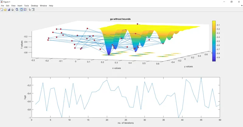
The above is the plotting section for the 'stalgmite_ga' function and the optimized value of the functions at the 'xopt' & 'yopt' optimized points.

The output of this plotting section can be seen in the screenshot as follows:

The first code

figure(1)

is for our plot must be in the 'figure(1)' window. Then we use the command

subplot(2,1,1)

as we want more than one plot in our 'figure(1)' window. As we want more than one plot in our 'figure(1)' window so we use more than one 'plot' command but the MATLAB will show the plot of the most recent 'plot' command, to avoid this we use the command

hold on

As I told you earlier that I want to visualize my function 'stalagmite_ga' in the form of a 3D surface so for that I use the command

surfc(xx,yy,f)

Under the parenthesis of this command, we insert the evaluated function & its input arrays. But the 3d surface from this command has grid lines and looks like a rough one so for a smoother-looking 3D surface, I use another command as

shading interp

with that colorful looking smoother 3D surface, I want a color bar also as it is convenient to visualize the z-coordinate through the colors so I use the command as

colorbar

I use the 'ga' which optimizes the 'stalagmite_ga' so the optimized value 'fopt' of this function at the points 'xopt' & 'yopt' are plotted with the 'marker' command with mark as 'o' of red color using the 'markerfacecolor' with 'r' under the parenthesis of this plot command, under the three axes (x,y,z) coordinate system so for that we use the

plot3(xopt,yopt,fopt,'marker','o','markerfacecolor','r')

command instead of the 'plot' command as it is used for only 2D axes system.

Now, if we want that our axes must be labeled so for that we need to use the commands 'xlabel', 'ylabel' & 'zlabel' as you can see the below code line with its format as:

xlabel('x values')
ylabel('y values')
zlabel('f values')

The written fonts or the names that you want on the axes are written in inverted commas under the parenthesis of these commands.

We have done all things which elaborate our plot of the figure window but again one question arises that this plot that we are seeing is for what and the answer is that this plot is for the minimizing value of our function using 'ga' without bounds so we can give a title to this plot of the figure window using the command as 'title' in a MATLAB format as can be seen below:

title('ga without bounds')

So I have completely explained the codings of the plots of this optimized 'stalagmite_ga' function but we have seen all in these in somewhat messy form so I want to show you the single plot of this evaluated & optimized function, for that, I use another

subplot(2,1,2)

command as in this same figure window. And that optimized function 'fopt' is plotted using the command

plot(fopt)

with the axes labels as

xlabel('no. of iterations')
ylabel('fopt')

This is about the 'ga' when it is without bounds (lb & ub) but when it is with the bounds such as lower bounds (lb) & upper bounds(ub) then how our 'ga' behaves? let's see

When 'ga' is with bounds such as lower bounds(lb) & upper bounds(ub)

% Defining the inputs of the function which we are going to optimize
x=linspace(0,0.6,200)
y=linspace(0,0.6,200)

% convert these input variables into 2D matrix
[xx, yy]=meshgrid(x,y)

num_cases=50


% Running a 'for loop' so that the values from 'xx' & 'yy' are taken & inserted into the inputs 'x' & 'y' of the function 
for i=1:length(xx)
for j=1:length(yy)
    input(1)=xx(i,j)
    input(2)=yy(i,j)
    f(i,j)=stalagmite_ga(input)
end    
end

% Configuring the 'ga' with the lower & upper bounds 
tic
for k=1:num_cases
    [inputs,fopt(k)]=ga(@stalagmite_ga,2,[],[],[],[],[0 0],[1 1])
    xopt(k)=inputs(1)
    yopt(k)=inputs(2)
end
bounded_ga=toc

% plotting
figure(2)
subplot(2,1,1)
hold on

surfc(xx,yy,f)
shading interp
colorbar

plot3(xopt,yopt,fopt,'marker','o','markerfacecolor','r')
xlabel('x values')
ylabel('y values')
zlabel('f values')
title('ga with bounds')

subplot(2,1,2)
plot(fopt)
xlabel('no. of iterations')
ylabel('fopt')

Now, I am explaining this case to you as:

% Defining the inputs of the function which we are going to optimize
x=linspace(0,0.6,200)
y=linspace(0,0.6,200)

The above coding section is for defining the inputs i.e., 'x' & 'y' of the function which we are going to call for the optimization purpose in this program using 'ga'.

% convert these input variables into 2D matrix
[xx, yy]=meshgrid(x,y)

num_cases=50

The above is the no. of cases or the no. of iterations for the running of 'ga'. here, it is '50' which means that our 'ga' runs 50 times.

% Running a 'for loop' so that the values from 'xx' & 'yy' are taken & inserted into the inputs 'x' & 'y' of the function 
for i=1:length(xx)
for j=1:length(yy)
    input(1)=xx(i,j)
    input(2)=yy(i,j)
    f(i,j)=stalagmite_ga(input)
end
end

Third code line under 'for loop' as

input(1)=xx(i,j)

input(2)=yy(i,j)

f(i,j)=stalagmite_ga(input)

So, finally under 'for loop', this function is gets evaluated and this function value will be in an array form so this 'stalagmite' function now can be visualized in a 3D surface form using the 'surfc' command.

% Configuring the 'ga' with the lower & upper bounds 
tic
for k=1:num_cases
    [inputs,fopt(k)]=ga(@stalagmite_ga,2,[],[],[],[],[0 0],[1 1])
    xopt(k)=inputs(1)
    yopt(k)=inputs(2)
end
bounded_ga=toc

Now, the above coding section is for the running of 'ga' for the optimization of our function 'stalagmite_ga'. As you know, I used the variable 'num_cases=50' which is for the running of 'ga' 50 times so for that I run a 'for loop' over this 'num_cases=50' which runs our 'ga' 50 times.

The 'ga' is used to minimize the function. In this above coding section, the 'ga' is configured with the lower & upper bounds(lb & ub) to visualize the performance of 'ga' which you will see when it is plotted in the plotting section when it is used with bounds.

Now, I am explaining to you the syntax of 'ga' that I used in this coding section:

[inputs,fopt(k)]=ga(@stalagmite_ga,2,[],[],[],[],[0 0],[1 1])

On R.H.S., you can see that we use the 'ga'. Under the parenthesis of 'ga', we insert the inputs of 'ga' as you can see we write '@stalagmite_ga' as we want to minimize the function 'stalagmite_ga' & with that we write '2' as we have two input variable of this function as 'x' & 'y' and with that we insert some boxes or square brackets also because the configuration of the inputs of 'ga' is predefined, so we can't randomly insert any input at any sequential order because the sequence of each of the inputs of the 'ga' is predetermined so we insert the lower '[0 0]' & upper [1 1] bounds on its predetermined place and leave the other square brackets as it is as you can see in the above-shown code line, even we can't remove the square brackets also.

Using the 'ga' with the bounds gives us the determined function optimized value under the limits of the bounds(lb & ub) that we have used.

 xopt(k)=inputs(1)
 yopt(k)=inputs(2)

So the first 'input(1)' is assigned to the variable 'xopt' & the second one 'input(2)' is assigned to the variable 'yopt'.

% plotting
figure(2)
subplot(2,1,1)
hold on

surfc(xx,yy,f)
shading interp
colorbar

plot3(xopt,yopt,fopt,'marker','o','markerfacecolor','r')
xlabel('x values')
ylabel('y values')
zlabel('f values')
title('ga with bounds')

subplot(2,1,2)
plot(fopt)
xlabel('no. of iterations')
ylabel('fopt')

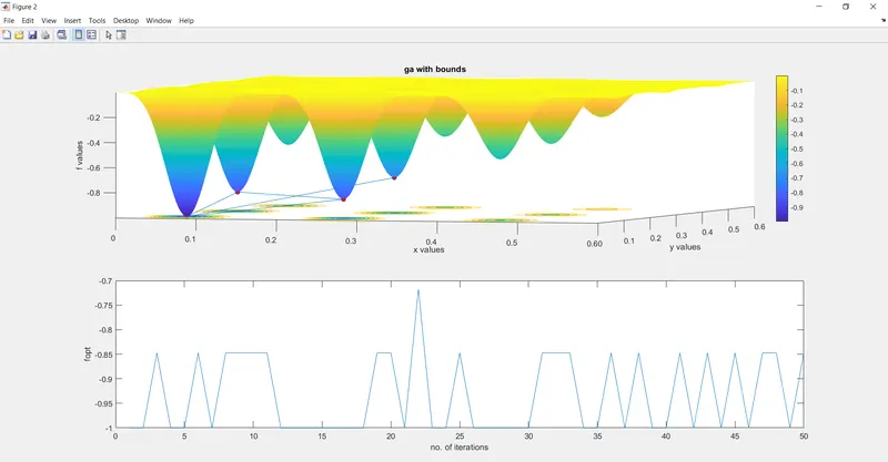
The above is the plotting section for the 'stalgmite_ga' function and the optimized value 'fopt' of the functions at the 'xopt' & 'yopt' optimized points.

The output of this plotting section can be seen in the screenshot as follows:

The first code

figure(1)

is for our plot must be in the 'figure(1)' window. Then we use the command

subplot(2,1,1)

hold on

As I told you earlier that I want to visualize my function 'stalagmite_ga' in the form of a 3D surface so for that I use the command

surfc(xx,yy,f)

shading interp

with that colorful looking smoother 3D surface, I want a color bar also as it is convenient to visualize the z-coordinate through the colors so I use the command as

colorbar

plot3(xopt,yopt,fopt,'marker','o','markerfacecolor','r')

command instead of the 'plot' command as it is used for only 2D axes system.

Now, if we want that our axes must be labeled so for that we need to use the commands 'xlabel', 'ylabel' & 'zlabel' as you can see the below code line with its format as:

xlabel('x values')
ylabel('y values')
zlabel('f values')

The written fonts or the names that you want on the axes are written in inverted commas under the parenthesis of these commands.

We have done all things which elaborate our plot of the figure window but again one question arises that this plot that we are seeing is for what and the answer is that this plot is for the minimizing value of our function using 'ga' with bounds so we can give a title to this plot of the figure window using the command as 'title' in a MATLAB format as can be seen below:

title('ga with bounds')

subplot(2,1,2)

command as in this same figure window. And that optimized function 'fopt' is plotted using the command

plot(fopt)

with the axes labels as

xlabel('no. of iterations')
ylabel('fopt')

This is about the 'ga' when it is with the bounds (lb & ub) but when it is with the bounds such as lower bounds (lb) & upper bounds(ub) as well as with the increase no. of iterations then how our 'ga' behaves? let's see

When 'ga' is with the bounds as well as with the increase in no. of population size

% Defining the inputs of the function which we are going to optimize
x=linspace(0,0.6,200)
y=linspace(0,0.6,200)

% convert these input variables into 2D matrix
[xx, yy]=meshgrid(x,y)


% Running a 'for loop' so that the values from 'xx' & 'yy' are taken & inserted into the inputs 'x' & 'y' of the function 
for i=1:length(xx)
for j=1:length(yy)
    input(1)=xx(i,j)
    input(2)=yy(i,j)
    f(i,j)=stalagmite_ga(input)
end
end


% Defining the 'ga' input 'options'(for optimization options) which consists the population size for 'ga'
options=optimoptions('ga')
options=optimoptions(options,'populationsize',200)

num_cases=50

% Configuring the 'ga' with bounds as well as with the 'options'(for optimization options)  
tic
for k=1:num_cases
    [inputs,fopt(k)]=ga(@stalagmite_ga,2,[],[],[],[],[0 0],[1 1],[],[],options)
    xopt(k)=inputs(1)
    yopt(k)=inputs(2)
end    
bounded_ga_with_increased_population_size=toc

% plotting
figure(3)
subplot(2,1,1)
hold on

surfc(xx,yy,f)
shading interp
colorbar

plot3(xopt,yopt,fopt,'marker','o','markerfacecolor','r')
xlabel('x values')
ylabel('y values')
zlabel('f values')
title('bounded ga with increased population size')

subplot(2,1,2)
plot(fopt)
xlabel('no. of iterations')
ylabel('fopt value')

Now, I am explaining this case to you as:

% Defining the inputs of the function which we are going to optimize
x=linspace(0,0.6,200)
y=linspace(0,0.6,200)

The above coding section is for defining the inputs i.e., 'x' & 'y' of the function which we are going to call for the optimization purpose in this program using 'ga'.

% convert these input variables into 2D matrix
[xx, yy]=meshgrid(x,y)

num_cases=50

The above is the no. of cases or the no. of iterations for the running of 'ga'. here, it is '50' which means that our 'ga' runs 50 times.

% Running a 'for loop' so that the values from 'xx' & 'yy' are taken & inserted into the inputs 'x' & 'y' of the function 
for i=1:length(xx)
for j=1:length(yy)
    input(1)=xx(i,j)
    input(2)=yy(i,j)
    f(i,j)=stalagmite_ga(input)
end
end

Third code line under 'for loop' as

input(1)=xx(i,j)

input(2)=yy(i,j)

f(i,j)=stalagmite_ga(input)

% Defining the 'ga' input 'options'(for optimization options) which consists the population size for 'ga'
options=optimoptions('ga')
options=optimoptions(options,'populationsize',200)

The above coding section is for defining the optimization options for 'ga' that we will use during configuring the 'ga' using the input 'options' that is why we first define it here. We use it here for increasing the population size for the optimization of our function 'stalagmite_ga' using 'ga'. As with the increase in population size, 'ga' gives a more accurate minimized value so we use it here.

I use the command 'optimoptions()' on the R.H.S. of the first code line and write 'ga' inside the parenthesis of this command as we want to optimize our function 'stalagmite_ga' using the chosen algorithm 'ga'. Then I again use the command 'optimoptions()' on R.H.S. in the next code line and as inputs in the parenthesis, I insert our created array variable 'options'(as in the first code line) with the 'population size' as I want to increase the population size up to '200' as you can see in the second code line of this section. Now, the array variable 'options' in the second code line consists of all the optimization options that I want so now, I can use this array 'options' while configuring the 'ga'.

tic
for k=1:num_cases
    [inputs,fopt(k)]=ga(@stalagmite_ga,2,[],[],[],[],[0 0],[1 1],[],[],options)
    xopt(k)=inputs(1)
    yopt(k)=inputs(2)
end    
bounded_ga_with_increased_population_size=toc

The 'ga' is used to minimize the function. In this above coding section, the 'ga' is configured with the lower & upper bounds(lb & ub) as well as with the 'options' (optimization options) to visualize the performance of 'ga' which you will see when it is plotted in the plotting section when it is used with bounds as well as with 'options' which consists the increased population size.

With all this, I want to calculate the compile time of the 'ga' so for that I use the 'tic' & 'toc' commands. I use the 'tic' command just before this 'for loop' and the 'toc' command which is assigned to the variable 'bounded_ga_with_increased_population_size' as here, 'ga' is with bounds with increased population size.

Now, I am explaining to you the syntax of 'ga' that I used in this coding section:

[inputs,fopt(k)]=ga(@stalagmite_ga,2,[],[],[],[],[0 0],[1 1],[],[],options)

On R.H.S., you can see that we use the 'ga'. Under the parenthesis of 'ga', we insert the inputs of 'ga' as you can see we write '@stalagmite_ga' as we want to minimize the function 'stalagmite_ga' & with that we write '2' as we have two input variable of this function as 'x' & 'y' and with that we insert some boxes or square brackets also because the configuration of the inputs of 'ga' is predefined, so we can't randomly insert any input at any sequential order because the sequence of each of the inputs of the 'ga' is predetermined so we insert the lower '[0 0]' & upper [1 1] bounds on its predetermined place as well as the array variable 'options' (which consists the optimized option as increased population size) at the last and leave the other square brackets as-it-is as you can see in the above-shown code line, even we can't remove the square brackets also.

Using the 'ga' with the bounds gives us the determined function optimized value under the limits of the bounds(lb & ub) that we have used and with the optimized option as increased population size in the array variable 'options' gives us the more converge optimized function value.

 xopt(k)=inputs(1)
 yopt(k)=inputs(2)

So the first 'input(1)' is assigned to the variable 'xopt' & the second one 'input(2)' is assigned to the variable 'yopt'.

% plotting
figure(3)
subplot(2,1,1)
hold on

surfc(xx,yy,f)
shading interp
colorbar

plot3(xopt,yopt,fopt,'marker','o','markerfacecolor','r')
xlabel('x values')
ylabel('y values')
zlabel('f values')
title('bounded ga with increased population size')

subplot(2,1,2)
plot(fopt)
xlabel('no. of iterations')
ylabel('fopt value')

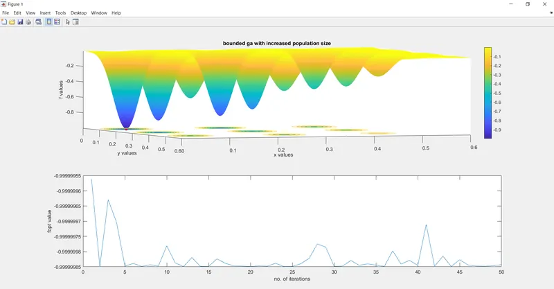
The above is the plotting section for the 'stalgmite_ga' function and the optimized value 'fopt' of the functions at the 'xopt' & 'yopt' optimized points.

The output of this plotting section can be seen in the screenshot as follows:

The first code

figure(3)

is for our plot must be in the 'figure(3)' window. Then we use the command

subplot(2,1,1)

as we want more than one plot in our 'figure(3)' window. As we want more than one plot in our 'figure(3)' window so we use more than one 'plot' command but the MATLAB will show the plot of the most recent 'plot' command, to avoid this we use the command

hold on

As I told you earlier that I want to visualize my function 'stalagmite_ga' in the form of a 3D surface so for that I use the command

surfc(xx,yy,f)

shading interp

with that colorful looking smoother 3D surface, I want a color bar also as it is convenient to visualize the z-coordinate through the colors so I use the command as

colorbar

plot3(xopt,yopt,fopt,'marker','o','markerfacecolor','r')

command instead of the 'plot' command as it is used for only 2D axes system.

Now, if we want that our axes must be labeled so for that we need to use the commands 'xlabel', 'ylabel' & 'zlabel' as you can see the below code line with its format as:

xlabel('x values')
ylabel('y values')
zlabel('f values')

The written fonts or the names that you want on the axes are written in inverted commas under the parenthesis of these commands.

We have done all things which elaborate our plot of the figure window but again one question arises that this plot that we are seeing is for what and the answer is that this plot is for the minimizing value of our function using bounded 'ga' with increased population size so we can give a title to this plot of the figure window using the command as 'title' in a MATLAB format as can be seen below:

title('bounded ga with increased population size')

subplot(2,1,2)

command as in this same figure window. And that optimized function 'fopt' is plotted using the command

plot(fopt)

with the axes labels as

xlabel('no. of iterations')
ylabel('fopt')

So finally, we find the global maxima of the function 'stalagmite_ga' at function value = '1' as you can see from the plot of figure(3) window of the attached file 'bounded_ga_with_increased_population_size' of the format (.fig).

So:

I attached the required MATLAB file of (.m) of the asked code.
I attached the codes with comments and explained them.
I attached the output plots of file format(.fig) & their screenshots for each case with proper labels & titles.

Explanations:

I explained the concept & theory of optimization & 'ga' from the information tab of the 'stalagmite mathematical model' video session as https://skill-lync.com/knowledgebase/genetic-algorithm-explained.
The stopping criteria of the 'ga' from https://www.tutorialspoint.com/genetic_algorithms/genetic_algorithms_termination_condition.htm
I explained the syntax of 'ga' in each case that I perform.
Also, I explained the significance of running multiple iterations.
I explained each case out of the 3 cases with its result in the explanation of the program.

So with the completion of all these, I am going to submit the report with the attachments.

Week 4.1 - Genetic Algorithm

Ship work like this
in your own course.

Talk to a career counsellor

Ship work like thisin your own course.

Talk to a career counsellor

Ship work like this
in your own course.