Project 2 - Rankine cycle Simulator

Rankine cycle:-

It is the cycle that runs in a Rankine engine proposed by 'William Johnson Macquorn Rankine'. This type of engine is used where the steam engine power plants are needed.

This engine consists of a Boiler, Turbine, Condenser, and Pump. Here, the working fluid is liquid & that working fluid is heated in a boiler at a higher temperature so that this fluid changes its phase from the liquid to the vapor. This vapor then enters the turbine blades through the turbine inlet where this fluid at high pressure & temperature strikes the blades to rotate them so that we can get a shaft output & that shaft is connected to the rotor of the rotor blades. This output is known as the work output of the turbine. After that this steam leaves the turbine through the turbine outlet & enters the condenser through the condenser inlet. In the condenser, the steam is cooled so that its phase gets changed to liquid water in order to reuse it as a working fluid. Now, this working fluid leaves the condenser through the condenser outlet and enters the pump where it is pumped or compressed at high pressure so that it can be reached the boiler & in the boiler it will be heated at high pressure and converted into a vapor or steam which can be used to rotate the rotor blades of the turbine & the cycle will go again & again like that.

It will be more clear when I will explain to you by my program 'RANKINE CYCLE SIMULATOR' as:

% RANKINE CYCLE SIMULATOR


clear all
close all
clc

% State 1
t1=400                   % given as Turbine inlet temperature
p1=30                    % given as Turbine inlet pressure   

% Reffering the XSteam table using programming
h1=XSteam('h_pT',p1,t1)  % 'h1' enthalpy at the Turbine inlet
s1=XSteam('s_ph',p1,h1)  % 's1' entropy at the Turbine inlet 


% State 2
p2=0.05                  % given as pressure at Turbine outlet or Condenser inlet
s2=s1                    % Isentropic expansion from state (1 to 2)
t2=XSteam('T_ps',p2,s2)  % Temperature 't2' at Turbine outlet or Condenser inlet

hf2=XSteam('hL_p',p2)
hg2=XSteam('hV_p',p2)
sf2=XSteam('sL_p',p2)
sg2=XSteam('sV_p',p2)

x2=((s2-sf2)/(sg2-sf2))  % 'x2' is the Dryness fraction

h2=hf2+(x2*(hg2-hf2))    % Enthalpy 'h2' at Turbine outlet or Condenser inlet



% State 3
p3=p2                    % Constant Pressure heat rejection from state (2 to 3)
t3=XSteam('Tsat_p',p3)   % 't3' temperature at Condenser outlet
h3=XSteam('hL_p',p3)     % 'h3' enthalpy at Condenser outlet
s3=XSteam('sL_p',p3)     % 's3' entropy at Condenser outlet




% State 4
s4=s3                    % Isentropic compression from state (3 to 4)
p4=p1                    % Constant pressure heat addition from state (4 to 1)


Cp=XSteam('CpL_p',p4)    % Specific heat capacity at constant pressure
Cv=XSteam('CvL_p',p4)    % Specific heat capacity at constant volume

gamma=Cp/Cv

T4=XSteam('T_ps',p4,s4)  % 't4' tempeature at Boiler inlet



V3=XSteam('v_ps',p3,s3)  % Volume of condensed liquid at Condenser outlet

Wp=V3*(p4-p3)*100        % Working of the pump
h4=h3+Wp                 % 'h4' enthalpy at Boiler inlet




% State point 5
% p4=p5=p6=p1 as of constant pressure heat addition from state (4 to 1)
p5=p1                    % Pressure 'p5' inside the boiler
s5=XSteam('sL_p',p5)     % 's5' entropy inside the Boiler
h5=XSteam('hL_p',p5)     % 'h5' enthalpy inside the Boiler
t5=XSteam('T_ph',p5,h5)  % 't5' temperature inside the Boiler



% State point 6
p6=p1                    % 'p6' pressure inside the Boiler
t6=t5                    % t6=t5 as can be seen in the T-S diagram of the project-2 as RANKINE CYCLE SIMULATION
h6=XSteam('hV_p',p6)     % 'h6' enthalpy of the working fluid inside the Boiler
s6=XSteam('sV_p',p6)     % 's6' entropy of the working fluid inside the Boiler


% Calculations:-
Wt=h1-h2                 % Working of turbine 
Wnet=Wt-Wp               % Net work output
Qin=h1-h4                % Heat input
Qout=h2-h3               % Heat output
Ntherm=Wnet/Qin          % Thermal efficiency
Wback=Wp/Wt              % Back work ratio

% Plotting of the T-S & H-S diagram of the Rankine cycle
figure(1)
plot(s1,t1,'*','color','r')  % Marking the state point 1 using the marker '*'
hold on
plot([s1 s2],[t1 t2],'linewidth',1,'color','r')  % Joining the state point (1 & 2)
plot(s2,t2,'*','color','y')  % Marking the state point 2 using the marker '*'

plot(s3,t3,'*','color','g')  % Marking the state point 3 using the marker '*'
plot([s3 s4],[t3 T4],'linewidth',2,'color','g')  % Joining the state point (3 & 4) 
plot(s4,T4,'*','color','b')  % Marking the state point 4 using the marker '*'

plot(s5,t5,'*','color','cyan')  % Marking the state point 5 using the marker '*'
plot([s5 s6],[t5 t6],'linewidth',1,'color','b')        % Joining the state point (5 & 6)
plot(s6,t6,'*','color','magenta')  % Marking the state point 6 using the marker '*'

plot([s2 s3],[t2 t3],'linewidth',1,'color','y')   % Joining the state point (2 & 3)
plot([s4 s5],[T4 t5],'linewidth',1,'color','b')   % Joining the state point (4 & 5)
plot([s6 s1],[t6 t1],'linewidth',1,'color','b')   % Joining the state point (6 & 1)


% Plotting of the T-S & H-S curves at liquid & vapour phases
t=linspace(0,400,100) % Making of the temperature array
for i=1:length(t)
    s_l(i)=XSteam('sL_T',t(i)) % Finding the entropy at liquid phase with the help of temperature array under 'for loop' using XSteam table
    s_V(i)=XSteam('sV_T',t(i)) % Finding the entropy at vapour phase with the help of temperature array under 'for loop' using XSteam table
end

plot(s_l,t)                    % T-S curve plot at liquid phase
plot(s_V,t)                    % T-S curve plot at vapour phase



title('T-S curve')        % Title of the plot/curve
xlabel('Entropy(S)')      % Labelling the entity name which is on the X-axis
ylabel('Temperature(t)')  % Labelling the entity name which is on the Y-axis

% Symbolise the curves as to show that which curve shows which process
legend('1 (Turbine)','1-2 isentropic expansion','2 (Condenser)','3 (Pump)','3-4 isentropic compression','4 (boiler)','5','5-6 vapourisation occurs at sat.temperature','6','2-3 isobaric heat rejection','4-1 isobaric heat addition','4-5','liquid phase curve','vapour phase curve')


figure(2)

plot(s1,h1,'*','color','r')  % Marking the state point 1 using the marker '*'  
hold on
plot(s2,h2,'*','color','g')  % Marking the state point 2 using the marker '*'
plot(s3,h3,'*','color','b')  % Marking the state point 3 using the marker '*'  
plot(s4,h4,'*','color','y')  % Marking the state point 4 using the marker '*'  

plot([s1 s2],[h1 h2])        % Joining the state points (1 & 2)
plot([s3 s4],[h3 h4])        % Joining the state points (3 & 4)

plot([s2 s3],[h2 h3])        % Joining the state points (2 & 3)
plot([s4 s1],[h4 h1])        % Joining the state points (4 & 1)



title('H-S curve')      % Title of the plot/curve
xlabel('Entropy(s)')    % Labelling the entity name which is on the X-axis
ylabel('Enthalpy(H)')   % Labelling the entity name which is on the Y-axis

% Symbolise the curves to show which curve shows which process
legend('1','2','3','4')


for i=1:length(t)
    h_L(i)=XSteam('hL_T',t(i)) % Finding the enthalpy at liquid phase with the help of temperature array under 'for loop' using XSteam table
    h_V(i)=XSteam('hV_T',t(i)) % Finding the enthalpy at vapour phase with the help of temperature array under 'for loop' using XSteam table
end
plot(s_V,h_V)                  % H-S curve plot at vapour phase

The above program 'RANKINE CYCLE SIMULATOR' is to simulate the Rankine cycle using its input data which will be used to analyze the performance & the efficiency of this cycle.

Now, I am explaining to you the each & every code of my program as follows:

(1).

clear all
close all
clc

With the above coding section, I initiate my program.

(2). We are dealing with the Rankine cycle, since a cycle consists of the state points & state variables so I determine the state points & its variable one by one using the given values & the variables in the Rankine cycle is 'pressure (p)', 'temperature (t)', 'entropy (s)', 'enthalpy (h)'. So the code for the state points is as follows:

% State 1
t1=400                   % given as Turbine inlet temperature
p1=30                    % given as Turbine inlet pressure   

% Reffering the XSteam table using programming
h1=XSteam('h_pT',p1,t1)  % 'h1' enthalpy at the Turbine inlet
s1=XSteam('s_ph',p1,h1)  % 's1' entropy at the Turbine inlet 

't1' & 'p1' are the given variables as can be read from the comments.

With the help of these given variables, I find out the other variables as 'h1' & 's1' using the 'XSteam table' as seen above. To find these from the 'XSteam table', there must be an XSteam program in the same folder. To find a variable from XSteam table, there is a command used in MATLAB for that & that is 'XSteam()'. for e.g., we have the pressure 'p1' & temperature 't1' & we want to find the enthalpy 'h1' at state point 1, so we use the command XSteam('h_pT',p1,t1). It is read as enthalpy as a function of pressure & temperature & which must be valid if it is in the 'XSteam table'.

(3).

% State 2
p2=0.05                  % given as pressure at Turbine outlet or Condenser inlet
s2=s1                    % Isentropic expansion from state (1 to 2)
t2=XSteam('T_ps',p2,s2)  % Temperature 't2' at Turbine outlet or Condenser inlet

hf2=XSteam('hL_p',p2)
hg2=XSteam('hV_p',p2)
sf2=XSteam('sL_p',p2)
sg2=XSteam('sV_p',p2)

x2=((s2-sf2)/(sg2-sf2))  % 'x2' is the Dryness fraction

h2=hf2+(x2*(hg2-hf2))    % Enthalpy 'h2' at Turbine outlet or Condenser inlet

The above coding section is for determining the variables of state 2 & which is at the outlet of the Turbine or the inlet of the condenser. It can be understood by the comments themselves as seen above. In the above codes, 'hf2' & 'hg2' are the enthalpies at the liquid & vapor phase at state point 2 respectively and 'sf2' & 'sg2' are the entropies at liquid & vapor phase respectively. And these are determined in order to find 'x2', the dryness fraction & 'h2', the enthalpy at state point 2.

(4).

% State 3
p3=p2                    % Constant Pressure heat rejection from state (2 to 3)
t3=XSteam('Tsat_p',p3)   % 't3' temperature at Condenser outlet
h3=XSteam('hL_p',p3)     % 'h3' enthalpy at Condenser outlet
s3=XSteam('sL_p',p3)     % 's3' entropy at Condenser outlet

The above is the coding section for finding the variables of state point 3. There is nothing to explain in this section as all things are explained by the comments themselves and I have explained the format of the command 'XSteam' in the 'state 1'.

(5).

% State 4
s4=s3                    % Isentropic compression from state (3 to 4)
p4=p1                    % Constant pressure heat addition from state (4 to 1)


T4=XSteam('T_ps',p4,s4)  % 't4' temperature at Boiler inlet



V3=XSteam('v_ps',p3,s3)  % Volume of condensed liquid at Condenser outlet

Wp=V3*(p4-p3)*100        % Working of the pump
h4=h3+Wp                 % 'h4' enthalpy at Boiler inlet

The above coding section is to determine the variables of the state point 4. These are the variables of the working fluid in the pump, and previously, I specified & explained the variables in the Rankine cycle state points. So that we have to find the pump work also. So you can see above the formula to find the pump work ('Wp').

In this state point, the new thing is that we have to find the volume at state point 3 i.e., 'V3' which is the variable of the formula, pump work ('Wp'). After finding the pump work('Wp'), with this pump work('Wp'), we can find the enthalpy 'h4' at this state point.

(5).

% State point 5
% p4=p5=p6=p1 as of constant pressure heat addition from state (4 to 1)
p5=p1                    % Pressure 'p5' inside the boiler
s5=XSteam('sL_p',p5)     % 's5' entropy inside the Boiler
h5=XSteam('hL_p',p5)     % 'h5' enthalpy inside the Boiler
t5=XSteam('T_ph',p5,h5)  % 't5' temperature inside the Boiler

The above is state point 5 which is at the boiler. So, I determined the variables of this state point as you can see above.

(6).

% State point 6
p6=p1                    % 'p6' pressure inside the Boiler
t6=t5                    % t6=t5 as can be seen in the T-S diagram of the project-2 as RANKINE CYCLE SIMULATION
h6=XSteam('hV_p',p6)     % 'h6' enthalpy of the working fluid inside the Boiler
s6=XSteam('sV_p',p6)     % 's6' entropy of the working fluid inside the Boiler

The above is state point 6 which is inside the boiler & undergoes the transition of the phase from liquid to the vapor. And I determine the variables of this state point as you can see above with the explanation using the comments with these variables.

(7).

% Calculations:-
Wt=h1-h2                 % Working of turbine 
Wnet=Wt-Wp               % Net work output
Qin=h1-h4                % Heat input
Qout=h2-h3               % Heat output
Ntherm=Wnet/Qin          % Thermal efficiency
Wback=Wp/Wt              % Back work ratio

Now, I am going to explain the above variables with their functions & calculations as follows:

Wt=h1-h2                 % Working of turbine 

The above is the Turbine work ('Wt') which is calculated by finding the differences in the enthalpies at the Turbine inlet & outlet respectively.

The use of a turbine in the Rankine cycle is to rotate the shaft connected to it & hence produce the output work. For this, the turbine also needs to be rotated which can be done by entering the high pressure & temperature steam into the rotor blades of the shaft & due to this high-pressure steam, the rotor blades of this turbine rotate & hence it will produce the output work in its turn.

Wnet=Wt-Wp               % Net work output

The above is the net work output & it is the difference between the turbine work & the pump work. For maximum net work, the difference between turbine work & pump work must be high, for that, the turbine work output must be greater & the pump work output must be lower so, for greater net work, their difference must be maximum so that we can get the maximum efficiency also.

Qin=h1-h4                % Heat input
Qout=h2-h3               % Heat output

The above is the heat input & heat output as can be seen. The heat input is the difference between the enthalpies at the boiler outlet & boiler inlet. Here, the liquid is boiled at a higher temperature inside the boiler to convert it into steam for the turbines and

the heat output is the difference between the enthalpies at the condenser inlet & condenser outlet. Here, the steam is condensed at a lower temperature to reuse this working fluid.

Ntherm=Wnet/Qin          % Thermal efficiency

The above is the thermal efficiency of this Rankine cycle. It is the ratio of the net work output to the heat input. It is the most important variable for any engine. It should be higher for any engine.

In general, efficiency itself means the ratio of the output to the input.

Wback=Wp/Wt              % Back work ratio

The above is the back work ratio which is defined as the ratio of the pump/compressor work to the turbine work.

(8).

% Plotting of the T-S & H-S diagram of the Rankine cycle
figure(1)
plot(s1,t1,'*','color','r')  % Marking the state point 1 using the marker '*'
hold on
plot([s1 s2],[t1 t2],'linewidth',1,'color','r')  % Joining the state point (1 & 2)
plot(s2,t2,'*','color','y')  % Marking the state point 2 using the marker '*'

plot(s3,t3,'*','color','g')  % Marking the state point 3 using the marker '*'
plot([s3 s4],[t3 T4],'linewidth',2,'color','g')  % Joining the state point (3 & 4) 
plot(s4,T4,'*','color','b')  % Marking the state point 4 using the marker '*'

plot(s5,t5,'*','color','cyan')  % Marking the state point 5 using the marker '*'
plot([s5 s6],[t5 t6],'linewidth',1,'color','b')        % Joining the state point (5 & 6)
plot(s6,t6,'*','color','magenta')  % Marking the state point 6 using the marker '*'

plot([s2 s3],[t2 t3],'linewidth',1,'color','y')   % Joining the state point (2 & 3)
plot([s4 s5],[T4 t5],'linewidth',1,'color','b')   % Joining the state point (4 & 5)
plot([s6 s1],[t6 t1],'linewidth',1,'color','b')   % Joining the state point (6 & 1)


% Plotting of the T-S & H-S curves at liquid & vapour phases
t=linspace(0,400,100) % Making of the temperature array
for i=1:length(t)
    s_l(i)=XSteam('sL_T',t(i)) % Finding the entropy at liquid phase with the help of temperature array under 'for loop' using XSteam table
    s_V(i)=XSteam('sV_T',t(i)) % Finding the entropy at vapour phase with the help of temperature array under 'for loop' using XSteam table
end

plot(s_l,t)                    % T-S curve plot at liquid phase
plot(s_V,t)                    % T-S curve plot at vapour phase



title('T-S curve')        % Title of the plot/curve
xlabel('Entropy(S)')      % Labelling the entity name which is on the X-axis
ylabel('Temperature(t)')  % Labelling the entity name which is on the Y-axis

% Symbolise the curves as to show that which curve shows which process
legend('1 (Turbine)','1-2 isentropic expansion','2 (Condenser)','3 (Pump)','3-4 isentropic compression','4 (boiler)','5','5-6 vapourisation occurs at sat.temperature','6','2-3 isobaric heat rejection','4-1 isobaric heat addition','4-5','liquid phase curve','vapour phase curve')


figure(2)

plot(s1,h1,'*','color','r')  % Marking the state point 1 using the marker '*'  
hold on
plot(s2,h2,'*','color','g')  % Marking the state point 2 using the marker '*'
plot(s3,h3,'*','color','b')  % Marking the state point 3 using the marker '*'  
plot(s4,h4,'*','color','y')  % Marking the state point 4 using the marker '*'  

plot([s1 s2],[h1 h2])        % Joining the state points (1 & 2)
plot([s3 s4],[h3 h4])        % Joining the state points (3 & 4)

plot([s2 s3],[h2 h3])        % Joining the state points (2 & 3)
plot([s4 s1],[h4 h1])        % Joining the state points (4 & 1)



title('H-S curve')      % Title of the plot/curve
xlabel('Entropy(s)')    % Labelling the entity name which is on the X-axis
ylabel('Enthalpy(H)')   % Labelling the entity name which is on the Y-axis

% Symbolise the curves to show which curve point shows which state point
legend('1','2','3','4')


for i=1:length(t)
    h_L(i)=XSteam('hL_T',t(i)) % Finding the enthalpy at liquid phase with the help of temperature array under 'for loop' using XSteam table
    h_V(i)=XSteam('hV_T',t(i)) % Finding the enthalpy at vapour phase with the help of temperature array under 'for loop' using XSteam table
end
plot(s_V,h_V)                  % H-S curve plot at vapour phase

The above is the plotting section of the program 'RANKINE CYCLE SIMULATOR' and this is the main section of this program as, without this, we can't analyze the data as the T-S curve & H-S curve. This section is lengthy so I explain this section part by part as follows:

(i).

% Plotting of the T-S & H-S diagram of the Rankine cycle
figure(1)
plot(s1,t1,'*','color','r')  % Marking the state point 1 using the marker '*'
hold on
plot([s1 s2],[t1 t2],'linewidth',1,'color','r')  % Joining the state point (1 & 2)
plot(s2,t2,'*','color','y')  % Marking the state point 2 using the marker '*'

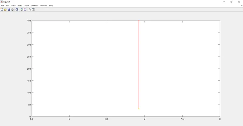
• This is the part of the plotting section by which I want to make the points as 1 & 2 for the state points 1 & 2 respectively and then join that points.
• The above plotting section is for the plotting of the state variables at state points (1 & 2) and the curve joining these points. Collectively, these state points and the curve joining these make a process and that process is known as the 'isentropic expansion process' in which the expansion of the volume of the steam occurs so in between the first & the last plot commands, we insert another plot command in between them which is for the joining of the state points at first & the third plot commands. So, this command 'plot' has the inputs as '[s1 s2]' & '[t1 t2]'.
• The first 'plot' command is used for plotting the state variables (s1,t1) as a marking point '*' at state point 1. So we put the input in the parenthesis as 's1', 't1', '*' with the desired color as red so we also use the 'color' command with the red color as 'r'. And these inputs under plot command must be put in this sequence if you use another sequence then it will be wrong and then MATLAB throws you an error in the 'command' window so here, the sequence matters.
• The third 'plot' command is used for plotting the state variables (s2,t2) as a marking point '*' at state point 2. So we put the input in the parenthesis as 's2', 't2', '*' with the desired color as yellow so we also use the 'color' command with the red color as 'y'. And these inputs under plot command must be put in this sequence if you use another sequence then it will be wrong and then MATLAB throws you an error in the 'command' window so here, the sequence matters.
• The second 'plot' command is used for joining the above-plotted state points like (1 & 2) to make a process that is 'isentropic expansion' as in this process, there is an expansion of the volume of the steam.

The output plot of the plotting section is shown in the below screenshot as follows:

(ii).

plot(s3,t3,'*','color','g')  % Marking the state point 3 using the marker '*'
plot([s3 s4],[t3 T4],'linewidth',2,'color','g')  % Joining the state point (3 & 4) 
plot(s4,T4,'*','color','b')  % Marking the state point 4 using the marker '*'

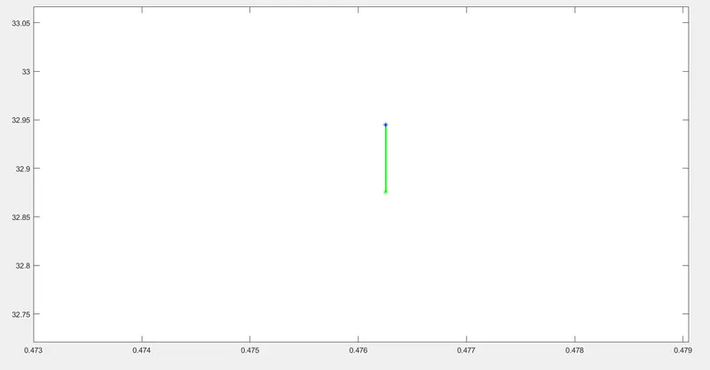
• This is the part of the plotting section by which I want to make the points 3 & 4 for the state points 3 & 4 respectively and then join that points.
• The above plotting section is for the plotting of the state variables at state points (3 & 4) and the curve joining these points. Collectively, these state points and the curve joining these make a process and that process is known as the 'isentropic compression process' in which the compression of the volume of the steam occurs in order to pass it to the inlet of the boiler so in between the first & the last plot commands, we insert another plot command in between them which is for the joining of the state points at first & the third plot commands. So, this command 'plot' has the inputs as '[s3 s4]' & '[t3 t4]'.
• The first 'plot' command is used for plotting the state variables (s3,t3) as a marking point '*' at state point 3. So we put the input in the parenthesis as 's3', 't3', '*' with the desired color as green so we also use the 'color' command with the green color as 'g'. And these inputs under plot command must be put in this sequence if you use another sequence then it will be wrong and then MATLAB throws you an error in the 'command' window so here, the sequence matters.
• The third 'plot' command is used for plotting the state variables (s4,t4) as a marking point '*' at state point 4. So we put the input in the parenthesis as 's4', 't4', '*' with the desired color as blue so we also use the 'color' command with the blue color as 'b'. And these inputs under plot command must be put in this sequence if you use another sequence then it will be wrong and then MATLAB throws you an error in the 'command' window so here, the sequence matters.
• The second 'plot' command is used for joining the above-plotted state points like (3 & 4) that makes a process that is 'isentropic compression' as in this process, there is a compression of the volume of the steam occurs to pass it into the boiler inlet.

The output plot of the plotting section is shown in the below screenshot as follows:

(iii).

plot(s5,t5,'*','color','cyan')  % Marking the state point 5 using the marker '*'
plot([s5 s6],[t5 t6],'linewidth',1,'color','b')        % Joining the state point (5 & 6)
plot(s6,t6,'*','color','magenta')  % Marking the state point 6 using the marker '*'

• This is the part of the plotting section by which I want to make the points 5 & 6 for the state points 5 & 6 respectively and then join that points.
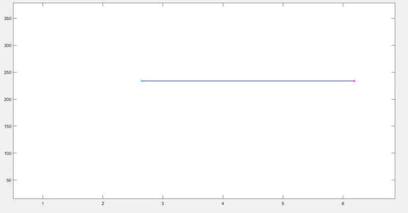
• The above plotting section is for the plotting of the state variables at state points (5 & 6) and the curve joining these points. Collectively, these state points and the curve joining these make a process and that process is known as the 'isobaric heat addition process' in which the addition of heat occurs to the steam at a constant pressure inside the boiler so in between the first & the last plot commands, we insert another plot command in between them which is for the joining of the state points at first & the third plot commands. So, this command 'plot' has the inputs as '[s5 s6]' & '[t5 t6]'.
• The first 'plot' command is used for plotting the state variables (s5,t5) as a marking point '*' at state point 5. So we put the input in the parenthesis as 's5', 't5', '*' with the desired color as cyan so we also use the 'color' command with the cyan color as 'cyan'. And these inputs under plot command must be put in this sequence if you use another sequence then it will be wrong and then MATLAB throws you an error in the 'command' window so here, the sequence matters.
• The third 'plot' command is used for plotting the state variables (s6,t6) as a marking point '*' at the state point 6. So we put the input in the parenthesis as 's6', 't6', '*' with the desired color as magenta so we also use the 'color' command with the magenta color as 'magenta'. And these inputs under plot command must be put in this sequence if you use another sequence then it will be wrong and then MATLAB throws you an error in the 'command' window so here, the sequence matters.
• The second 'plot' command is used for joining the above-plotted state points like (5 & 6) that makes a process that is 'isobaric heat addition' as in this process, the heat is given at a constant pressure to the steam inside the boiler.

The output plot of the plotting section is shown in the below screenshot as follows:

(iv).

plot([s2 s3],[t2 t3],'linewidth',1,'color','y')   % Joining the state point (2 & 3)
plot([s4 s5],[T4 t5],'linewidth',1,'color','b')   % Joining the state point (4 & 5)
plot([s6 s1],[t6 t1],'linewidth',1,'color','b')   % Joining the state point (6 & 1)

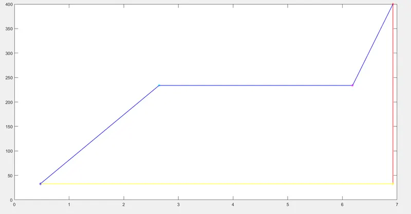
• The above plotting section is for the joining of the state variables at state points (2 & 3),(4 & 5), and (6 & 1). Collectively, these state points (2 to 3) and the curve joining these make a process and that process is known as the 'isobaric heat rejection' process in which the heat is rejected inside the condenser and the other process from the state point (4 to 1) is the 'isobaric heat addition' process in which the heat is added to the steam inside the boiler.

The output of this T-S plotting section is as follows:

(V).

% Plotting of the T-S & H-S curves at liquid & vapour phases
t=linspace(0,400,100) % Making of the temperature array
for i=1:length(t)
    s_l(i)=XSteam('sL_T',t(i)) % Finding the entropy at liquid phase with the help of temperature array under 'for loop' using XSteam table
    s_V(i)=XSteam('sV_T',t(i)) % Finding the entropy at vapour phase with the help of temperature array under 'for loop' using XSteam table
end

plot(s_l,t)                    % T-S curve plot at liquid phase
plot(s_V,t)                    % T-S curve plot at vapour phase

The above part of the plotting section is for the continuous T-S curve to the liquid as well as to the vapor side as the phase transition occurs as follows:

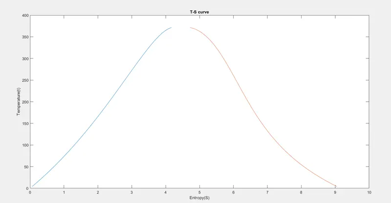
• The blue curve is on the liquid region while the brown curve is on the vapor region.
• This is the toughest task of this challenge as to how to obtain the above curve as an output?
• Because to obtain this above curve, the first question arises, Which concept of MATLAB is used here? & then how to use that concept?
• The answer to that is the 'for loop' must be used here because this curve is continuous in nature so we need each & every point of the temperature as well as the entropy and we have given temperature so we make an array of the temperature & with the help of this temperature array, I am going to find the entropies at the liquid as well as the vapor phase.
• Now, the question arises that how to find the entropies at this phase with the help of the temperature array?
• The answer to this is the XSteam table where all the variables can be calculated as a function of others so here I use this 'XSteam()' command in the 'for loop' for the entropies at the liquid as well as at the vapor region as can be seen in the above coding section. And then on finding the entropies, I plot this T-S curve as entropies ('S') & temperature ('t') on the X-axis & Y-axis respectively.

Now, the complete output plot of the H-S plotting section is as follows:

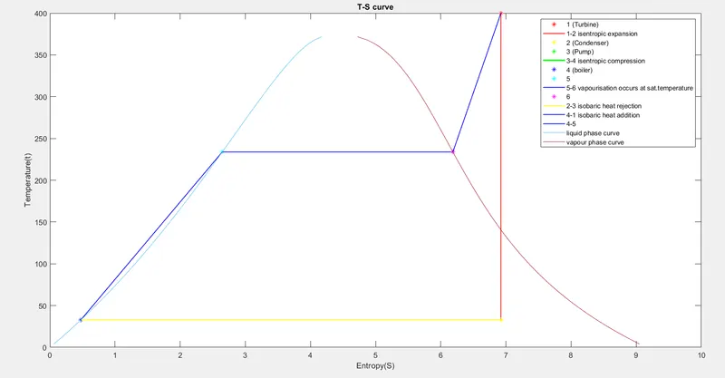
(vi).

title('T-S curve')        % Title of the plot/curve
xlabel('Entropy(S)')      % Labelling the entity name which is on the X-axis
ylabel('Temperature(t)')  % Labelling the entity name which is on the Y-axis

% Symbolise the curves as to show that which curve shows which process
legend('1 (Turbine)','1-2 isentropic expansion','2 (Condenser)','3 (Pump)','3-4 isentropic compression','4 (boiler)','5','5-6 vapourisation occurs at sat.temperature','6','2-3 isobaric heat rejection','4-1 isobaric heat addition','4-5','liquid phase curve','vapour phase curve')

The above section is the specification of the plotting curves as the name or title of the curve for that I use the 'title()' command, the data on the X-axis as well as on the Y-axis for that I use the commands as 'xlabel()' & 'ylabel()' respectively, there is more than one curve in a single figure window so I use the 'legend()' command whose inputs contains the state points as well as the processes under which these curves passes.

(vii).

figure(2)

plot(s1,h1,'*','color','r')  % Marking the state point 1 using the marker '*'  
hold on
plot(s2,h2,'*','color','g')  % Marking the state point 2 using the marker '*'
plot(s3,h3,'*','color','b')  % Marking the state point 3 using the marker '*'  
plot(s4,h4,'*','color','y')  % Marking the state point 4 using the marker '*'  

plot([s1 s2],[h1 h2])        % Joining the state points (1 & 2)
plot([s3 s4],[h3 h4])        % Joining the state points (3 & 4)

plot([s2 s3],[h2 h3])        % Joining the state points (2 & 3)
plot([s4 s1],[h4 h1])        % Joining the state points (4 & 1)

The above is the part of the plotting section to plot the H-S curve. The H-S curve has four state point & the four curve which joins these state points so first, I code for these state points as follows:

plot(s1,h1,'*','color','r')  % Marking the state point 1 using the marker '*'  
hold on
plot(s2,h2,'*','color','g')  % Marking the state point 2 using the marker '*'
plot(s3,h3,'*','color','b')  % Marking the state point 3 using the marker '*'  
plot(s4,h4,'*','color','y')  % Marking the state point 4 using the marker '*'  

• The first 'plot' command is used for plotting the state variables (s1,h1) as a marking point '*' at state point 1. So we put the input in the parenthesis as 's1', 'h1', '*' with the desired color as red so we also use the 'color' command with the red color as 'r'. And these inputs under plot command must be put in this sequence if you use another sequence then it will be wrong and then MATLAB throws you an error in the 'command' window so here, the sequence matters.
• The second 'plot' command is used for plotting the state variables (s2,h2) as a marking point '*' at state point 2. So we put the input in the parenthesis as 's2', 'h2', '*' with the desired color as green so we also use the 'color' command with the green color as 'g'. And these inputs under plot command must be put in this sequence if you use another sequence then it will be wrong and then MATLAB throws you an error in the 'command' window so here, the sequence matters.
• The third 'plot' command is used for plotting the state variables (s3,h3) as a marking point '*' at state point 3. So we put the input in the parenthesis as 's3', 'h3', '*' with the desired color as blue so we also use the 'color' command with the blue color as 'b'. And these inputs under plot command must be put in this sequence if you use another sequence then it will be wrong and then MATLAB throws you an error in the 'command' window so here, the sequence matters.
• The fourth 'plot' command is used for plotting the state variables (s4,h4) as a marking point '*' at state point 1. So we put the input in the parenthesis as 's4', 'h4', '*' with the desired color as yellow so we also use the 'color' command with the yellow color as 'y'. And these inputs under plot command must be put in this sequence if you use another sequence then it will be wrong and then MATLAB throws you an error in the 'command' window so here, the sequence matters.

The output plot of the plotting section is shown in the below screenshot as follows:

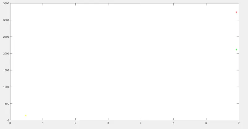
Now, I code for the joining of these state points as follows:

plot([s1 s2],[h1 h2])        % Joining the state points (1 & 2)
plot([s3 s4],[h3 h4])        % Joining the state points (3 & 4)

plot([s2 s3],[h2 h3])        % Joining the state points (2 & 3)
plot([s4 s1],[h4 h1])        % Joining the state points (4 & 1)

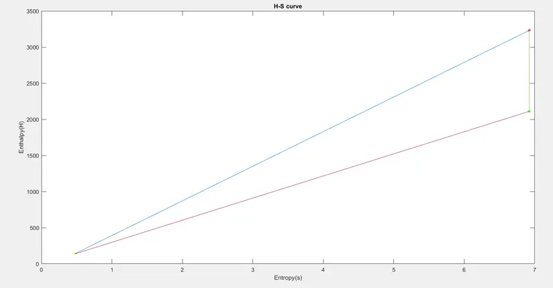
• The above plotting section is for the joining of the state variables at state points (1 & 2),(3 & 4), (2 & 3), and (4 & 1).
• Collectively, these state points (1 to 2) and the curve joining these make a process and that process is known as the 'isentropic expansion' process in which the volume of the steam is expanded inside the turbine.
• The state points (3 to 4) and the curve joining these make a process and that process is known as the 'isentropic compression' process in which the volume of the steam is compressed inside the pump.
• The state points (2 to 3) and the curve joining these make a process and that process is known as the 'isobaric heat rejection' process in which the heat is rejected from the steam & is condensed into liquid in the condenser.
• The state points (4 to 1) and the curve joining these make a process and that process is known as the 'isobaric heat addition' process in which the heat is added to the liquid & is boiled into the vapor in the boiler.

The output plot of this plotting section is shown in the below screenshot as follows:

(viii).

for i=1:length(t)
    h_L(i)=XSteam('hL_T',t(i)) % Finding the enthalpy at liquid phase with the help of temperature array under 'for loop' using XSteam table
    h_V(i)=XSteam('hV_T',t(i)) % Finding the enthalpy at vapour phase with the help of temperature array under 'for loop' using XSteam table
end
plot(s_V,h_V)                  % H-S curve plot at vapour phase

The above part of the plotting section is for the continuous H-S curve to the vapor region of the Rankine cycle as follows:

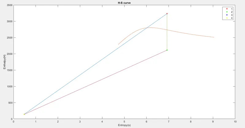
• The free curve which is not linear as you can see is the curve on the vapor region is from the above coding section.
• And this section is to plot the H-S curve.
• This is the toughest task of this challenge as to how to obtain the above curve as an output?
• Because to obtain this above curve, the first question arises, Which concept of MATLAB is used here? & then how to use that concept?
• The answer to that is the 'for loop' must be used here because this curve is continuous in nature so we need each & every point of the enthalpy as well as the entropy and we have given temperature so with the help of the temperature array that I made & with the help of this temperature array, I am going to find the enthalpies at the vapor phase as I had found the entropies in the previous section.
• Now, the question arises that how to find the enthalpies at this phase with the help of the temperature array?
• The answer to this is the XSteam table where all the variables can be calculated as a function of others so here I use this 'XSteam()' command in the 'for loop' for the enthalpies at the vapor region as can be seen in the above coding section. And then on finding the enthalpies, I plot this H-S curve as enthalpy ('H') & entropy ('S') on the X-axis & Y-axis respectively.

(ix).

title('H-S curve')      % Title of the plot/curve
xlabel('Entropy(s)')    % Labelling the entity name which is on the X-axis
ylabel('Enthalpy(H)')   % Labelling the entity name which is on the Y-axis

% Symbolise the curves to show which curve point shows which state point
legend('1','2','3','4')

The above section is the specification of the plotting curves as the name or title of the curve for that I use the 'title()' command, the data on the X-axis as well as on the Y-axis for that I use the commands as 'xlabel()' & 'ylabel()' respectively, there is more than one curve in a single figure window so I use the 'legend()' command whose inputs contains the state points as ('1', '2', '3', '4').

So:

• I Create a Rankine Cycle Simulator using OCTAVE/MATLAB.
• My code calculates the state points of the Rankine Cycle based on the inputs.
• Then, I plot the corresponding T-s and h-s plots for the given set of inputs with the title and axes labels and with the legends also as there are multiple curves in a single figure window.
• I label my coding sections using the comments.
• With all that I make a report which explains the Rankine cycle simulator & I attached it.
• I also calculate the following as

1. Net work output
2. Back work ratio

So, by completing all the objectives of this project 2- RANKINE CYCLE SIMULATOR, I am going to submit this.