Week 3 - Solving second order ODEs

Problem: Write a program in Matlab that will simulate the pendulum motion.

Solution: For that, I have to first solve the ODE of a moving pendulum then use this solved ODE in MATLAB in a coding format to make a program using the concept of 'function' so it will be a 'defined function' which I named as 'Function of the solved ODE of the moving pendulum' and attached as a file named as 'ode_func' of the file format (.m). And use this 'defined function' by calling its input parameters with its function name in our main program which I named 'Simulation of the oscillating pendulum by using its simple ODE'so that we can obtain the simulation of this moving pendulum animatedly as an output. And the youtube link to this animation video is as follows:

https://youtu.be/iE-pjKRT0wQ

              first, we need to make a function & defined it, and call this function in our main program as I mentioned previously.

              So These are the following codes that I used in my function 'Function of the solved ODE of the moving pendulum' as follows:

function [dtheta_dt]=ode_func(t,theta,b,g,l,m)
    theta1=theta(1);
    theta2=theta(2);
    dtheta1_dt=theta2;
    dtheta2_dt=(-b/m)*theta2-(g/l)*sin(theta1);
    dtheta_dt=[dtheta1_dt;dtheta2_dt];
end

            Now, I am explaining to you each & every code of this defined function as follows:

function [dtheta_dt]=ode_func(t,theta,b,g,l,m)

            Our function starts from this above-shown code line with the starting code as 'function'. On R.H.S., 'ode_func' is the name of this function with its input parameters in the parenthesis as you can see above. And this is assigned to the variable 'dtheta_dt' which is the output variable of this function. So to define this function, we have to define this output variable. And this output variable is defined in the second last code line. So under this function, we define our output variable which is nothing but our function definition.

             For understanding purpose, we use the bottom to top approach:

(i). 

dtheta_dt=[dtheta1_dt;dtheta2_dt]

             The above code line is for defining the output variable which is on the L.H.S. of this above code line to define this function. The above code line is written based on the solution of the ODE of the moving pendulum. So this code line not only defines our output variable but is also known to be the solution matrice in this MATLAB function as it is the solution of our ODE of the moving pendulum.

             On L.H.S., of this coding, we have 'dtheta_dt' which is our output variable.

             On R.H.S., of this code, we defined this output variable as under the square brackets as [dtheta1_dt;dtheta2_dt] which I will explain to you in the next points as follows.

(a). 

dtheta1_dt=theta2
dtheta2_dt=(-b/m)*theta2-(g/l)*sin(theta1)

              As you can see the L.H.S. of the above code lines, 'dtheta1_dt' & 'dtheta2_dt' are the R.H.S. terms of our defined output. For complete defining, we define these variables also as you can see in the above code lines. Now, we need to define the R.H.S. variable of the above code lines. As the variables 'b', 'g', 'l', 'm' are the input variables we can't define them as they are used during the calling of this function with the function name but the variables 'theta1' & 'theta2' are not input parameters so we define them in the next points as follows.

(b).  

 theta1=theta(1)
 theta2=theta(2)

             As you can see the above code lines are used to define 'theta1' & 'theta2' as 'theta(1)' & 'theta(2)' respectively which are nothing but the angular displacements and the angular velocities of the oscillating pendulum at different instants of time respectively. These are obtained during the calling of this function in our main program which you can see in the array named as 'results' in the workspace of our main program.

end

          We end our function using the command 'end'. Without this command, our function is incomplete and it is not said to be as a function.

          Now, we use this above function for calling in our main program named 'Simulation of the oscillating pendulum by using its simple ODE' and the codes of this main program that we use are as follows:

% Simulation of the oscillating pendulum by using its simple ODE  


close all
clc

% inputs
b=0.05;
g=9.81;
l=1;
m=1;



% initial conditions
theta_0=[0;3];

% Time integration
t_span=linspace(0,20,100);

% calling the function using the MATLAB solver
[t,results]=ode45(@(t,theta)ode_func(t,theta,b,g,l,m),t_span,theta_0);

% Position Coordinates
x0=0;
y0=0;



ct=1;
for i=1:length(t_span)
    results(i,1);

x1=l*cos(results(i,1));
y1=l*sin(results(i,1));

% Plotting for the animation parameters
figure(2)
hold on

% Rigid fixed bar of the oscillating pendulum
plot([0,0],[-1,1],'linewidth',3,'color','g')
% Pivit point of the pendulum
plot(x0,y0,'o','markerfacecolor','y','markeredgecolor','y')
% For making an string of the pendulum
line([x0 x1],[y0 y1],'linewidth',1,'color','b')
% For showing the ball/bob with a finite size using the 'marker'
plot(x1,y1,'o','markersize',10,'markerfacecolor','r','markeredgecolor','r')


% For labelling the x-axis with the running parameter on it
xlabel('x displacement')
% For labelling the y-axis with the running parameter on it
ylabel('y displacement')

% For giving the title to the animation
title('Simulation of a pendulum under damping')

% Making an array of all the frames for the making of an animating file 
M(ct)=getframe(gcf);
ct=ct+1;
grid on
end

% Making of the animation file
movie(M)
videofile=VideoWriter('pendulum simulations.avi','Uncompressed AVI');
open(videofile)
writeVideo(videofile,M)
close(videofile)


% plotting of the curves of the entities of the output 'results' w.r.t. 't'
figure(1)
plot(t,results(:,1),'linewidth',1,'color','r')
hold on
plot(t,results(:,2),'linewidth',1,'color','b')

% For labelling the x-axis with the running parameter on it
xlabel('time (t)')

% For labelling the y-axis with the running parameter on it
ylabel('Oscillations (results)')

% For giving the title to the plot of the 'figure' window
title('Damping of the pendulum oscillations w.r.t. time')

% To distinguish the curves in the plot 
legend('angular displacement','angular velocity')

                Now, I explain each & every code of this main program with its output in the screenshot as follows:

(1). 

close all
clc

% inputs
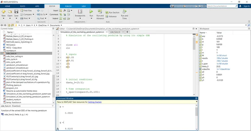
b=0.05;
g=9.81;
l=1;
m=1;

          The above coding section is the initiation of our main program using the function call. I am explaining the code lines of this section point by point as follows:

(i). 

close all
clc

           The first two codes 'close all' & 'clc' can/can't be used (not compulsory) but I used as during initiation if there is any window like 'figure' opened then it will be closed automatically by using the code 

close all

and if there is anything displayed or printed as an output in the command window then it will be cleared by using the code 

clc

(ii). 

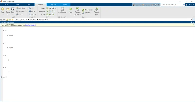
b=0.05

             For MATLAB, the term 'b' is nothing but just a code that is a variable & is assigned for a scalar no. '0.05' as can be seen in the above coding.

             We define the input parameter 'b' of the defined function that I explained above as we are going to call this function in this our main program so I define this above shown input parameter as for calling purpose.  Here the variable 'b' refers to the damping coefficient.

             In the terms of a mechanical engineer, the word 'damping' has a lot to do. 

             Damping is defined as the resistance to the vibration of an oscillating body. It has wide applications in the field of designing the spring-in-the-damper system. Because using the concept of damping, we design the dampers to prevent the excessive oscillations of the spring in the spring-damper system.

(ii). 

g=9.81

               For MATLAB, the term 'g' is nothing but just a code that is a variable & is assigned for a scalar no. '9.81' as can be seen in the above coding.

               We define the input parameter 'g' of the defined function that I explained above as we are going to call this function in this our main program so I define this above shown input parameter as for calling purpose.  Here the variable 'g' refers to the gravitational constant.

               In the terms of a mechanical engineer, the word 'gravitation' has a lot to do. 

               Gravitation is defined as the downward force/pull towards the earth's surface. This is a physical phenomenon that is everywhere as we lived on the planet 'earth'.

               We can't control this phenomenon but we can balance this phenomenon by using our mechanical skills. 

(iii). 

l=1

                For MATLAB, the term 'l' is nothing but just a code that is a variable & is assigned for a scalar no. '1' as can be seen in the above coding.

                We define the input parameter 'l' of the defined function that I explained above as we are going to call this function in this our main program so I define this above shown input parameter as for calling purpose.  Here the variable 'l' refers to the length of the string of the pendulum.

(iv). 

m=1

                 For MATLAB, the term 'm' is nothing but just a code that is a variable & is assigned for a scalar no. '1' as can be seen in the above coding.  

                  We define the input parameter 'm' of the defined function that I explained above as we are going to call this function in this our main program so I define this above shown input parameter as for calling purpose.  Here the variable 'm' refers to the mass of the ball/bob of the pendulum.

              The output in the 'command' window of the above coding section is shown in the following screenshot:      

       

       

(2). 

% initial conditions
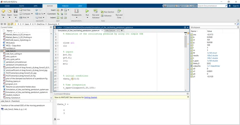
theta_0=[0;3]

                    The above coding is for defining the initial condition of the pendulum.

                    On L.H.S., 'theta_0' is the variable that is an array for the initial condition of the ball of the pendulum which consists of the initial displacement & initial velocity of the ball as of '0' & '3' respectively which can be seen on the R.H.S. of the above coding.

                    The logic behind this coding is that for the simulation of an oscillating pendulum, we need to define its initial conditions/parameters as the oscillating body possesses its displacement & maybe velocity also w.r.t. time(t) so we need to specify its displacement & velocity at 't=0'. This is a mathematical method that is used for both analytical as well as computational purposes.

               The output in the 'command' window of this above code line is shown in the following screenshot:      

         

(3). 

% Time integration
t_span=linspace(0,20,100)

                     The above coding is for the integration of our input parameters in between a time span/limit of '0' to '20' with '100' values as you can see in the parenthesis on the R.H.S. of the above coding.

                     The logic behind the above coding is that we deal with the ODE of the oscillating pendulum. So this oscillating pendulum has different positions at different instants of time so for animating simulation we need to integrate or bind these different instants of time together to get an animation. Also for analytical purposes, when we deal with situations of the moving systems with ODEs, we need the integration of an appropriate parameter in between the time span/limits. That's why we use the codes of time integration such as 't_span'. 

                    The variable 't_span' is an array of '100' values as you can see above in the parenthesis so it is inconvenient to show its output in the form of a screenshot.

(4). 

% calling the function using the MATLAB solver
[t,results]=ode45(@(t,theta)ode_func(t,theta,b,g,l,m),t_span,theta_0)

                     The above code line is for calling the ODE function using the MATLAB solver 'ode45'. We use the MATLAB solver 'ode45' because we are calling the function whose output variable is in the form of an ODE solution. If its output variable is not an ODE solution then we can't use this MATLAB solver because this MATLAB solver is inbuilt which is built for such ODEs solutions.

                      Now, I am explaining to you the above whole format and we can't change this format as it is created by MATLAB so we have to use this same format when needed.

                      So for calling an ODE function with the MATLAB solver 'ODE45', we start from the L.H.S. as 

                     '[t,y]' here our y is 'results' and on R.H.S., we use the MATLAB solver 'ode45' with its input under the parenthesis as you can see above. 

                      As you can see above, Under the parenthesis, '@(t, theta)' are the main inputs of this MATLAB solver 'ode45', and then we call our function (that I have explained previously) under this same parenthesis as an input of this MATLAB solver 'ode45' and at last we pass on time integration as well as the initial conditions as 't_span' & 'theta_0' respectively.

(5). 

% Position Coordinates
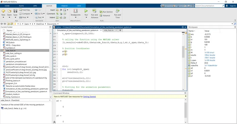
x0=0
y0=0

                       The above codes are the position coordinates of the hinge point of the pendulum. As we are coding for the simulation of a moving pendulum so we need to define each & every coordinate of the pendulum as a pendulum consists of a rigid bar, hinge point, pendulum string, ball/bob at the end of the string. So we have to define the coordinates of all these parts of this moving pendulum. 

                    The output in the 'command' window of this above coding is shown in the following screenshot: 

         

(6). 

ct=1;
for i=1:length(t_span)
    results(i,1);

x1=l*cos(results(i,1));
y1=l*sin(results(i,1));

% Plotting for the animation parameters
figure(2)
hold on

% Rigid fixed bar of the oscillating pendulum
plot([0,0],[-1,1],'linewidth',3,'color','g')
% Pivit point of the pendulum
plot(x0,y0,'o','markerfacecolor','y','markeredgecolor','y')
% For making an string of the pendulum
line([x0 x1],[y0 y1],'linewidth',1,'color','b')
% For showing the ball/bob with a finite size using the 'marker'
plot(x1,y1,'o','markersize',10,'markerfacecolor','r','markeredgecolor','r')


% For labelling the x-axis with the running parameter on it
xlabel('x displacement')
% For labelling the y-axis with the running parameter on it
ylabel('y displacement')

% For giving the title to the animation
title('Simulation of a pendulum under damping')

% Making an array of all the frames for the making of an animating file 
M(ct)=getframe(gcf);
ct=ct+1;
grid on
end

                     The above coding section is for running a 'for loop' for the angular displacement of the pendulum so that we can see the moving/oscillating pendulum during the simulation.

ct=1

                    As you can see above that before the 'for loop', we initiate the counter ('ct=1') which is just a code used to initiate the frame for the animation, and then the 'for loop'  starts.

                    The output of this above code in the 'command' window can be shown in the following screenshot:

        

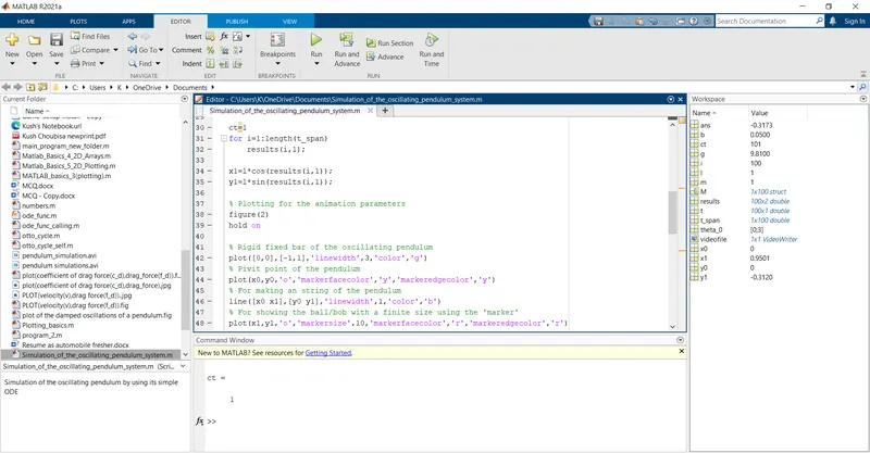
                    Now, I am explaining the coding sections under 'for loop' as follows:

for i=1:length(t_span)

 Here, 'i' is the loop operator of this 'for loop' as the loop operator 'i' is used to execute the codes under this 'for loop' (with the same loop operator) at many times with different assigned values at each time with each value out of the different assigned values.

                Here, you can see that on the R.H.S. of loop operator 'i', it is written as '1:length(t_span)' which means that the loop operator 'i' operates the 'for loop' from '1' to the 'length(t_span)', as 'length(t_span)' is nothing, it is just the total no. of contained values in the array 't_span'. Here, in this program 'length('t_span') is equal to '100' as 't_span' contains hundred values. So the loop operator 'i' operates the 'for loop' 100 times.

(ii). 

 results(i,1)

             We want to run a 'for loop' for 'results(i,1)' that is for every row of the 'first' column of the array 'results' to change its values automatically using programming.  We need to change each & every value of 'results(i,1)' that's why we use the loop operator 'i' instead of a constant number at the place of row inside the parenthesis of the array 'results'. So that this loop operator 'i' changes at every execution of the 'for loop' and it changes to each value of the row of the first column of the array 'result' at each & every execution/run of this 'for loop'. 

             The logic behind this coding is that we can change each & every value of the angular displacement (which is the first column of the array 'results') so that we can trace the angular displacement of the pendulum w.r.t. the time 't' which results in the simulation of the pendulum as an oscillating pendulum.    

(iii). 

x1=l*cos(results(i,1))
y1=l*sin(results(i,1))

               The above code lines are the (x,y) position coordinates of the ball/bob of the pendulum.

               And these coordinates are obtained using trigonometric ratios from the geometry of the path traced by the oscillating pendulum. And its output in the 'command' window is much bigger as it has the array 'results' so I didn't attach the screenshot of the output for convenience. 

               The logic behind the above coding is that under the 'for loop', at every run of the loop, the value of the loop operator 'i' changes which result in the change of the value of this above position coordinates as it also contains the loop operator 'i' under the parenthesis so that at every different time we get the different position of the pendulum ball which is nothing but just the movement of this pendulum ball in an oscillation manner.

(iv). 

% Plotting for the animation parameters
figure(2)
hold on

% Rigid fixed bar of the oscillating pendulum
plot([0,0],[-1,1],'linewidth',3,'color','g')
% Pivit point of the pendulum
plot(x0,y0,'o','markerfacecolor','y','markeredgecolor','y')
% For making an string of the pendulum
line([x0 x1],[y0 y1],'linewidth',1,'color','b')
% For showing the ball/bob with a finite size using the 'marker'
plot(x1,y1,'o','markersize',10,'markerfacecolor','r','markeredgecolor','r')


% For labelling the x-axis with the running parameter on it
xlabel('x displacement')
% For labelling the y-axis with the running parameter on it
ylabel('y displacement')

% For giving the title to the animation
title('Simulation of a pendulum under damping')

                  The above coding section is for plotting the oscillating/moving pendulum under the 'for loop'.  

(a). 

figure(2)

                   Under this section, we use the above code 'figure(2)' as we want our simulation from this code under the frame/ figure window as 'figure2'.

(b). 

hold on

                   The above command is used when we plot more than one curve. This command line is used when we use the plotting commands for more than one curve as we want to make a plot as output that has '4' curves, so use more than one plot command. If we don't use the above-shown command then the MATLAB will show the output of the most recent plot command so to prevent this we use this above-shown command as we want the output of each & every plot command. 

(c). 

% Rigid fixed bar of the oscillating pendulum
plot([0,0],[-1,1],'linewidth',3,'color','g')

                    This 'plot' command is used for the plotting line on the y-axis as '[0,0],[-1,1] since the x-coordinate on the y-axis is 0 so we put the endpoint's input of x-coordinates as '[0,0]' and we can put any desired coordinates of y-axis as here we put as '[-1,1]'. And this line is the rigidly fixed bar of our oscillating pendulum.

                    When using the plot command with its input as x & y coordinates in the parenthesis then the MATLAB first expects the x-coordinates of that plotting curve and then its y-coordinates as can be seen in the above code line. And then we use the line specification using commands 'linewidth' for the desired width of the line, here we want as '3' and the command 'color' for the desired color of the line, here we want it as 'g' stands for green color. 

                     The output of this above plotting curve line is can be seen in the following screenshot:

(d). 

% Pivit point of the pendulum
plot(x0,y0,'o','markerfacecolor','y','markeredgecolor','y')

                    The above 'plot' command is used for plotting the pivot point of this pendulum and since the pivot point is can be of the circular/spherical shape so for such type of plotting, we use the 'markers' which can be chosen based on the shape of the plotting entity as you can see above, we use 'o' as a marker but before that, we put the XY-coordinates where we plot that plotting entity here we plot it at origin as 'x0,y0' and with the plotting of this if we want the desired color of the face & edge of the marker then we use the commands as 'markerfacecolor' & 'markeredgecolor' respectively as you can see above.

(e). 

% For making an string of the pendulum
plot([x0 x1],[y0 y1],'linewidth',1,'color','b')

                   This 'plot' command is used for plotting the line/string of the pendulum and the XY-coordinates of this line curve as '[x0 x1]', '[y0 y1]' which can be seen above in the parenthesis. This plot is the most important in this program because without this plot we can't see the animating simulation of this pendulum as the inputs XY-coordinates (x1) & (y1) of this plot curve contains the loop operator 'i' without that we can't run the 'for loop' for the each & every value of the angular displacement under the array 'results'.

                    When using the plot command with its input as x & y coordinates in the parenthesis then the MATLAB first expects the x-coordinates of that plotting curve and then its y-coordinates as can be seen in the above code line. And then we use the line specification using commands 'linewidth' for the desired width of the line, here we want as '1' and the command 'color' for the desired color of the line, here we want it as 'b' stands for blue color.   

(f). 

% For showing the ball/bob with a finite size using the 'marker'
plot(x1,y1,'o','markersize',10,'markerfacecolor','r','markeredgecolor','r')

                 The above 'plot' command is used for plotting the ball/bob of this pendulum and since the ball/bob is can be of the circular/spherical shape so for such type of plotting, we use the 'markers' which can be chosen based on the shape of the plotting entity as you can see above, we use 'o' as a marker but before that, we put the XY-coordinates where we plot that plotting entity here we plot it at origin as 'x1,y1' and these coordinates runs under the 'for loop' as it runs using the loop operator 'i' which is nothing but each & every value of angular displacement which runs at each compilation with each value under the loop operator 'i' and without this above code line we can't see the simulation of the ball of the pendulum and with the plotting of this if we want the desired color of the face & edge of the marker then we use the commands as 'markerfacecolor' & 'markeredgecolor' respectively as you can see above.  

(g). 

% For labelling the x-axis with the running parameter on it
xlabel('x displacement')
% For labelling the y-axis with the running parameter on it
ylabel('y displacement')

                 The above command line is for labeling/naming the axes (x & Y). So for that, we use the 'label' command. So for X-axis, we write the first code line with 'x displacement' as an input under the parenthesis of xlabel as well as

for Y-axis, we write the second code line with 'y displacement' as an input under the parenthesis of ylabel. 

(h). 

% Making an array of all the frames for the making of an animating file 
M(ct)=getframe(gcf)
ct=ct+1

                  The above coding section is for making an array of all the frames so on running the code, these frames run after each other and we got the simulation as an animating video.

M(ct)=getframe(gcf)

             The above code line is used when we want to make an animation or movie of the simulating program. We can analyze the simulating program without the movie or animation but the problem is that for simulation of the program, we used the 'pause()' command which pauses the program again & again which decreases the performance of the program so we make an animation of the simulating program to stop the usage of the 'pause()' command.

         Here, in the above code line, 'ct' is an array that contains all the frames or figures windows which all are used to make an animation video so for collecting all the frames, the array 'ct' is assigned to a variable 'M'.

 Note:  for all this, we need to define 'ct=1' to initiate the frame and it is done before the 'for loop'.

          And on R.H.S., 'getframe()' is a command of MATLAB which is used to get all the frames with the parenthesis under which we put our input, here our input in the form of 'figure' windows for which we wrote 'gcf' inside the parenthesis.

ct=ct+1

         And after all this, we need to increment the 'ct' by 1 so as 'ct=ct+1' as can be seen from the above code line. So that during simulation, each & every frame gets executed/run one by one after each other.

        But the above code line should be written inside the 'for loop'. If not, then the simulation will not occur as each & every frame is obtained when the values of the parameters change automatically using 'for loop' so the increment of 'ct' which consists of all the frames must be done inside the 'for loop'.

(I). 

grid on

        For grids in the 'figure' window of the plot, we use this above command as 'grid on', if we don't use this command then grids will not be shown in the 'figure' window. 

(j). 

end

        The above code 'end' is used to end/complete the 'for loop'. Without this, there will be no 'for loop'  so we can't run a loop that's why we use the command 'end' at the end of the 'for loop'.

(7). 

% Making of the animation file
movie(M)
videofile=VideoWriter('pendulum simulations.avi','Uncompressed AVI');
open(videofile)
writeVideo(videofile,M)
close(videofile)

           The above code lines are used to make a file of a movie/animation.

           That's why on the first code line, we use the inbuilt code 'movie' to which we give input as an array 'M' to play the movie of all the collected frames in the array 'M'.

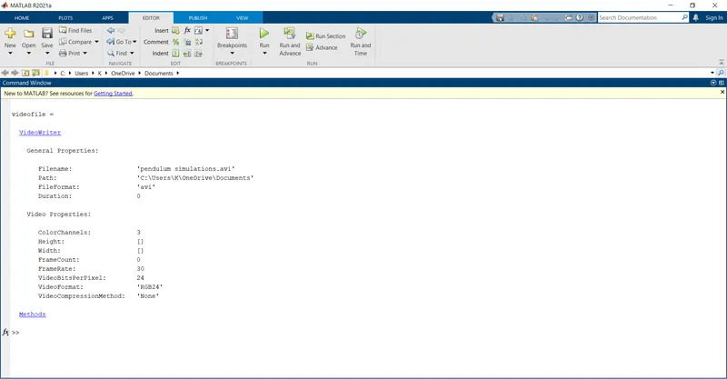
videofile=VideoWriter('pendulum simulations.avi','Uncompressed AVI');

            The above code line is used to make the file of the animating video so we used the command 'VideoWriter()' on R.H.S. to make the video file of the animating video, that's why we assign this to the variable as 'videofile' on R.H.S. 

            The command 'VideoWriter()' is with the parenthesis is used to make an animating file. The parenthesis with this is used to put an input inside it. And the inputs to this command are the 'file name' and the 'profile' of the file.

            As can be seen from the above code line that the file name is 'pendulum simulations.avi' & the profile is 'uncompressed AVI'. When we run this above code line then its output on the 'command' window gives us the description of the video file as can be seen from the below screenshot:

        

open(videofile)

          The above command 'open()' is used to add the functionality of opening to the file which is written as an input in the parenthesis with the 'open' command. Here, the input is the name of the file 'videofile'.

writeVideo(videofile,M)

           The above command 'writeVideo()' with inputs in the parenthesis is used to write the frames in the file name of your video so that as an input in the parenthesis, we put the file name under which we write the frames which are collected in the array 'M'. That's why we put inputs as 'videofile,M' inside the parenthesis as an input.

close(videofile)

           We make the animation file named 'videofile' using the command 'VideoWriter()' with the file name & its profile as the inputs.

            After the making of this file, we need to open the file so we add the functionality of open using the command 'open()' with the input as a file name.

            After opening the file, we need to write the frames in the file so we use the command 'writeVideo()' with the file name & array of frames as the inputs. So we can play this video file.

            Now, after playing the file, we need to close the file so we add the functionality of closing the file using the command 'close()' with the file name as an input.

(8). 

% plotting of the curves of the entities of the output 'results' w.r.t. 't'
figure(1)
plot(t,results(:,1),'linewidth',1,'color','r')
hold on
plot(t,results(:,2),'linewidth',1,'color','b')

% For labelling the x-axis with the running parameter on it
xlabel('time (t)')

% For labelling the y-axis with the running parameter on it
ylabel('Oscillations (results)')

% For giving the title to the plot of the 'figure' window
title('Damping of the pendulum oscillations w.r.t. time')

% To distinguish the curves in the plot 
legend('angular displacement','angular velocity')

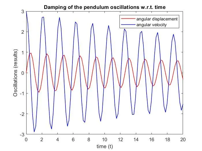
               The above coding section is for plotting the curves for angular displacement & angular velocity of the oscillating pendulum w.r.t. time 't'. The output of this plotting section is shown in the following screenshot:

 

(i). 

figure(1)

               Under this section, we use the above code 'figure(1)' as we want our simulation from this code under the frame/ figure window as 'figure1'.

(ii). 

plot(t,results(:,1),'linewidth',1,'color','r')
hold on
plot(t,results(:,2),'linewidth',1,'color','b')

                The first line 'plot' command with its inputs in the parenthesis is used for plotting the curve of the angular displacement w.r.t. time 't' as can be seen above that 't' is in place of the x coordinate and the y coordinate is the array 'results' which contains the two columns with one is the values of angular displacement the other is the value of angular velocity respectively but here we take the first column as a curve plotting of the angular displacement.

                So for the plotting of the angular displacement & angular velocities, we need to choose the appropriate column. For angular displacement, we choose the first column and for angular velocity, we choose the second column as can be seen in the above code lines for plotting.

                 The third line 'plot' command with its inputs in the parenthesis is used for plotting the curve of the angular velocity w.r.t. time 't' as can be seen above that 't' is in place of the x coordinate and the y coordinate is the array 'results' which contains the two columns with one is the values of angular displacement the other is the value of angular velocity respectively but here we take the second column as a curve plotting of the angular velocity.

                  On the second code line, we use the 'hold on' command. This command is used when we plot more than one curve. This command line is used when we use the plotting commands for more than one curve as we want to make a plot as output that has '2' curves, so use more than one plot command. If we don't use the above-shown command then the MATLAB will show the output of the most recent plot command so to prevent this we use this above-shown command as we want the output of each & every plot command.  

(iii). 

% For labelling the x-axis with the running parameter on it
xlabel('time (t)')

% For labelling the y-axis with the running parameter on it
ylabel('Oscillations (results)')

                 The above command line is for labeling/naming the axes (x & Y). So for that, we use the 'label' command. So for X-axis, we write the first code line with 'time (t)' as an input under the parenthesis of xlabel as well as

for Y-axis, we write the second code line with 'Oscillations (results)' as an input under the parenthesis of ylabel. 

(iv).

% For giving the title to the plot of the 'figure' window
title('Damping of the pendulum oscillations w.r.t. time')

                  The above code line is for giving the title to the plot of the 'figure' window. As you can see above for giving the title we use the command 'title()' with the parenthesis under which we put our title as you can see above.

(v).   

% To distinguish the curves in the plot 
legend('angular displacement','angular velocity')

                  The above code line is used as we are plotting more than one curve under the same 'figure' window so for distinguishing as well as naming we use the above-shown command as 'legend()' with the parenthesis under which we name these curves so when we see the output plot, we can distinguish the curve with the data/information for which the curve is displaying.

                   Actually, during the writing of this program & function, I got unaware of the errors in the report & forget to take screenshots of the errors that I got so that, I am not mentioning the errors, my bad, so next time, I will be aware for this & mention all the errors with their screenshots at 'command' window.

           So, according to me

      (i). I attached the codes with their comments. 

     (ii). I attached the pendulum animation with proper labels & title.

     (iii). So I explained the coding logic, the syntax of ode45, and the loop to create animation in detail.

So with all these, I completed my report on the challenge 'Solving second order ODEs' and going to submit this.