Challenge

Week 7 - Simulation of a 1D Supersonic nozzle flow simulation using Macormack Method

SSuhail Ahmed S3 Dec 2023

SIMULATION OF A 1D-SUPERSONIC NOZZLE FLOW SIMULATION USING MACCORMACK METHOD

Aim:

To stimulate a 1D-supersonic nozzle flow simulation using maccormack method for both conservation and non-conservation form of governing equations.

Objectives:

Need to show the following plots in the report

Steady-state distribution of primitive variables inside the nozzle.
Time-wise variation of primitive variables.
Variation of mass flow rate distribution inside the nozzle at the different time steps during the time-marching process.
Comparison of Normalized mass flow rate distributions of both forms.

Expected results:

Perform a grid independence test on the solution and explain all your findings.
The code must be modular. You need to write separate functions to solve both forms.
Discuss all the plots you are providing with observed inferences.

Theory:

A nozzle is a relatively simple device, just a specially shaped tube through which hot gases flow. Ramjets and rockets typically use a fixed convergent section followed by a fixed divergent section for the design of the nozzle. This nozzle configuration is called as convergent-divergent or CD nozzle.

In a CD nozzle, the hot exhaust leaves the combustion chamber and converges down to the minimum area or throat of the nozzle. The throat size is chosen to choke the flow and set the mass flow rate through the system. The flow in the throat is sonic which means the Mach number is equal to one in the throat. Downstream of the throat, the geometry diverges and the flow is isentropically expanded to a supersonic Mach number that depends on the area ratio of the exit to the throat.

The expansion of a supersonic flow causes the static pressure and temperature to dercrease from the throat to the exit, so the amount of the expansion also determines the exit pressure and temperature. The exit temperature determines the exit speed of sound, which determines the exit velocity. The exit velocity, pressure, and mass flow through the nozzle determines the amount of thrust produced by the nozzle.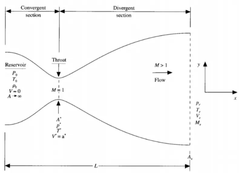Maccormack Method:

In computational fluid dynamics,the Maccormack method is a widely used discretization scheme for the numerical solution of hyperbolic partial differential equations.The maccormack method is elegant and easy to understand and program.

In general the maccormack method involves a "predictor step" and a "corrector step".

Predictor step: In a predictor step, a "provisional" value of u at time step n+1 as follows

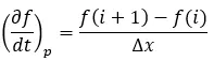
2. Solution update: In this initial values is updated.

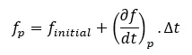
3. Corrector step: In the corrector step, the predictor value is updated according to the equation

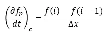
4. Average value: The average values of predictor and corrector time step

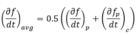
5. Final value update: Final solution of the first time step.

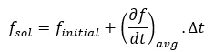Governing Equation:

The governing equation is solved using maccormack method for both forms conservative and non-conservative forms.

Conservative Equations:

1. Continuity Equation:

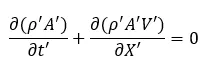2. Momentum Equation:

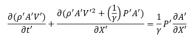3. Energy Equation:

Non-Conservative Equations:

1. Continuity Equation:

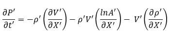
2. Momentum Equation:

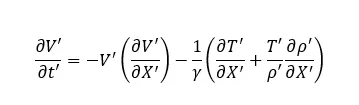
3. Energy Equation:

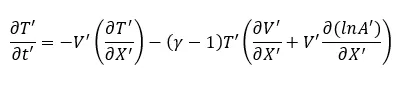
Matlab Codes:

Main code:

The main code is written for both function codes used to solve the 1D Quasi supersonic nozzle.

%1D QUASI SUPERSONIC NOZZLE FLOW

clear all

close all

clc

%Inputs

n = 31; %No. of grid points

gamma = 1.4;

x = linspace(0,3,n);

dx = x(2) - x(1);

nt = 1400; %No. of time step

C = 0.5; %Courant Number

%FUNCTION CALL FOR NON CONSERVATIVE EQUATIONS

tic;

[Mass_flow_rate_NC, Pressure_NC, Mach_number_NC, rho_NC, v_NC, T_NC, rho_throat_NC, v_throat_NC, T_throat_NC, Mass_flow_rate_throat_NC, Pressure_throat_NC, Mach_number_throat_NC] = non_conservative(x, dx, n, gamma, nt, C);

Time_elapsed_NC = toc;

fprintf('Time Elasped for Non Conservative form: %0.4f', Time_elapsed_NC);

hold on

%Plots

figure(2)

%Timestep variation of properties at throat area (Non-Conservative form)

%Density

subplot(4,1,1)

plot(linspace(1,nt,nt),rho_throat_NC,'color','c')

ylabel('Density')

legend({'Density at throat'});

axis([0 1400 0 1.3]);

grid minor;

title('Timestep variation at throat area - NON CONSERVATIVE FORM')

%Temperature

subplot(4,1,2)

plot(linspace(1,nt,nt),T_throat_NC,'color','r')

ylabel('Temperature')

legend({'Temperature at throat'});

axis([0 1400 0.6 1]);

grid minor;

%Pressure

subplot(4,1,3)

plot(linspace(1,nt,nt),Pressure_throat_NC,'color','g')

ylabel('Pressure')

legend({'Pressure at throat'});

axis([0 1400 0.4 1.1]);

grid minor;

%Mach Number

subplot(4,1,4)

plot(linspace(1,nt,nt),Mach_number_throat_NC,'color','y')

xlabel('Timesteps')

ylabel('Mach Number')

legend({'Mach Number at throat'});

axis([0 1400 0.6 1.4]);

grid minor;

figure(3);

%Steady state simulation for primitive values (Non-Conservative form)

%Density

subplot(4,1,1);

plot(x,rho_NC,'color','c')

ylabel('Density')

legend({'Density'});

axis([0 3 0 1])

grid minor;

title('Variation of Flow Rate Distribution - NON CONSERVATIVE')

%Temperature

subplot(4,1,2);

plot(x,T_NC,'color','r')

ylabel('Temperature')

legend({'Temperature'});

axis([0 3 0 1])

grid minor;

%Pressure

subplot(4,1,3);

plot(x,Pressure_NC,'color','g')

ylabel('Pressure')

legend({'Pressure'});

axis([0 3 0 1])

grid minor;

%Mach number

subplot(4,1,4);

plot(x,Mach_number_NC,'color','y')

xlabel('Nozzle Length')

ylabel('Mach number')

legend({'Mach number'});

axis([0 3 0 4])

grid minor;

%FUNCTION CALL FOR CONSERVATIVE FORM

tic;

[Mass_flow_rate_C, Pressure_C, Mach_number_C, rho_C, v_C, T_C, rho_throat_C, v_throat_C, T_throat_C, Mass_flow_rate_throat_C, Pressure_throat_C, Mach_number_throat_C] = conservative(x, dx, n, gamma, nt, C);

Time_elasped_C = toc;

fprintf('Time Elasped for Conservative form: %0.4f', Time_elasped_C);

%Plots

figure(5)

%Timestep variation of properties at throat area (Conservative form)

%Density

subplot(4,1,1)

plot(rho_throat_C,'color','c')

ylabel('Density')

legend({'Density at throat'});

axis([0 1400 0 1]);

grid minor;

title('Timestep variation at throat area - CONSERVATIVE FORM')

%Temperature

subplot(4,1,2)

plot(T_throat_C,'color','r')

ylabel('Temperature')

legend({'Temperature at throat'});

axis([0 1400 0.6 1]);

grid minor;

%Pressure

subplot(4,1,3)

plot(Pressure_throat_C,'color','g')

ylabel('Pressure')

legend({'Pressure at throat'});

axis([0 1400 0.2 0.8]);

grid minor;

%Mach Number

subplot(4,1,4)

plot(Mach_number_throat_C,'color','y')

xlabel('Timesteps')

ylabel('Mach Number')

legend({'Mach Number at throat'});

axis([0 1400 0.6 1.4]);

grid minor;

figure(6);

%Steady state simulation for primitive values (Conservative form)

%Density

subplot(4,1,1);

plot(x,rho_C,'color','c')

ylabel('Density')

legend({'Density'});

axis([0 3 0 1])

grid minor;

title('Variation of Flow Rate Distribution - CONSERVATIVE FORM')

%Temperature

subplot(4,1,2);

plot(x,T_C,'color','r')

ylabel('Temperature')

legend({'Temperature'});

axis([0 3 0 1])

grid minor;

%Pressure

subplot(4,1,3);

plot(x,Pressure_C,'color','g')

ylabel('Pressure')

legend({'Pressure'});

axis([0 3 0 1])

grid minor;

%Mach number

subplot(4,1,4);

plot(x,Mach_number_C,'color','y')

xlabel('Nozzle Length')

ylabel('Mach number')

legend({'Mach number'});

axis([0 3 0 4])

grid minor;

figure(7)

%Mass Flow Rate Comparison Plot

hold on

plot(x,Mass_flow_rate_NC,'r','linewidth',1)

hold on;

plot(x,Mass_flow_rate_C,'b','linewidth',1)

hold on;

grid on

legend('Non Conservative','Conservative');

xlabel('Length of the Domain')

ylabel('Mass Flow Rate')

title('Comparison of Mass Flow Rate of both forms')

Function code for Non-conservative form:

%Function code for Non-Conservative form

function [Mass_flow_rate_NC, Pressure_NC, Mach_number_NC, rho_NC, v_NC, T_NC, rho_throat_NC, v_throat_NC, T_throat_NC, Mass_flow_rate_throat_NC, Pressure_throat_NC, Mach_number_throat_NC] = non_conservative(x, dx, n, gamma, nt, C)

%Initial boundary conditions

rho_NC = 1 - 0.3146*x;

T_NC = 1 - 0.2341*x;

v_NC = (0.1 + 1.09*x).*T_NC.^0.5;

a = 1 + 2.2*(x - 1.5).^2; %Area profile

throat = find(a==1); %Throat profile

%Outer Time Loop

for k = 1:nt

%Time-step control

dt = min(C.*dx./(sqrt(T_NC) + v_NC));

%Saving a copy of Old Values

rho_old = rho_NC;

T_old = T_NC;

v_old = v_NC;

%Step 1 - Predictor method (forward difference for space terms)

for j = 2:n-1

%Simplifying the Equation's spatial terms

dv_dx = (v_NC(j + 1) - v_NC(j))/dx;

drho_dx = (rho_NC(j + 1) - rho_NC(j))/dx;

dT_dx = (T_NC(j + 1) - T_NC(j))/dx;

dlog_a_dx = (log(a(j + 1)) - log(a(j)))/dx;

%Continuity Equation

drho_dt_P(j) = -rho_NC(j)*dv_dx - rho_NC(j)*v_NC(j)*dlog_a_dx - v_NC(j)*drho_dx;

%Momentum Equation

dv_dt_P(j) = -v_NC(j)*dv_dx - (1/gamma)*(dT_dx + (T_NC(j)*drho_dx/rho_NC(j)));

%Energy Equation

dT_dt_P(j) = -v_NC(j)*dT_dx - (gamma - 1)*T_NC(j)*(dv_dx + v_NC(j)*dlog_a_dx);

%Step 2 - Solution update

rho_NC(j) = rho_NC(j) + drho_dt_P(j)*dt;

v_NC(j) = v_NC(j) + dv_dt_P(j)*dt;

T_NC(j) = T_NC(j) + dT_dt_P(j)*dt;

end

%Step 3 - Corrector method (backward difference for space terms)

for j = 2:n-1

%Simplifying the Equation's spatial terms

dv_dx = (v_NC(j) - v_NC(j - 1))/dx;

drho_dx = (rho_NC(j) - rho_NC(j - 1))/dx;

dT_dx = (T_NC(j) - T_NC(j - 1))/dx;

dlog_a_dx = (log(a(j)) - log(a(j - 1)))/dx;

%Continuity Equation

drho_dt_C(j) = - rho_NC(j)*dv_dx - rho_NC(j)*v_NC(j)*dlog_a_dx - v_NC(j)*drho_dx;

%Momentum Equation

dv_dt_C(j) = - v_NC(j)*dv_dx - (1/gamma)*(dT_dx + (T_NC(j)*drho_dx/rho_NC(j)));

%Energy Equation

dT_dt_C(j) = - v_NC(j)*dT_dx - (gamma - 1)*T_NC(j)*(dv_dx + v_NC(j)*dlog_a_dx);

end

%Step 4 - finding Average derivatives

drho_dt = 0.5.*(drho_dt_P + drho_dt_C);

dv_dt = 0.5.*(dv_dt_P + dv_dt_C);

dT_dt = 0.5.*(dT_dt_P + dT_dt_C);

%Step 5 - Final solution update

for i = 2:n-1

rho_NC(i) = rho_old(i) + drho_dt(i)*dt;

v_NC(i) = v_old(i) + dv_dt(i)*dt;

T_NC(i) = T_old(i) + dT_dt(i)*dt;

end

%Applying Boundary Conditions

%At Inlet

rho_NC(1) = 1;

v_NC(1) = 2*v_NC(2) - v_NC(3);

T_NC(1) = 1;

%At Outlet

rho_NC(n) = 2*rho_NC(n-1) - rho_NC(n - 2);

v_NC(n) = 2*v_NC(n - 1) - v_NC(n - 2);

T_NC(n) = 2*T_NC(n - 1) - T_NC(n - 2);

%Defining Mass flow rate, Pressure and Mach number

Mass_flow_rate_NC = rho_NC.*a.*v_NC;

Pressure_NC = rho_NC.*T_NC;

Mach_number_NC = (v_NC./sqrt(T_NC));

%Calculating Variables at throat section

rho_throat_NC(k) = rho_NC(throat);

T_throat_NC(k) = T_NC(throat);

v_throat_NC(k) = v_NC(throat);

Mass_flow_rate_throat_NC(k) = Mass_flow_rate_NC(throat);

Pressure_throat_NC(k) = Pressure_NC(throat);

Mach_number_throat_NC(k) = Mach_number_NC(throat);

%PLOTTING

%Comparison of non-dimensional Mass flow rates at different time steps

figure(1);

if k == 50

plot(x, Mass_flow_rate_NC, 'y', 'linewidth', 1);

hold on

elseif k == 100

plot(x, Mass_flow_rate_NC, 'g', 'linewidth', 1);

hold on

elseif k == 200

plot(x, Mass_flow_rate_NC, 'r', 'linewidth', 1);

hold on

elseif k == 400

plot(x, Mass_flow_rate_NC, 'c', 'linewidth', 1);

hold on

elseif k == 800

plot(x, Mass_flow_rate_NC, 'k', 'linewidth', 1);

hold on

end

%Labelling

title('Mass flow rates at different Timesteps - NON CONSERVATIVE FORM')

xlabel('Distance')

ylabel('Mass flow rate')

legend({'50^t^h Timestep','100^t^h Timestep','200^t^h Timestep','400^t^h Timestep','800^t^h Timestep'})

axis([0 3 0 2])

grid on

end

Function code for Conservative form:

%Function code for Conservative form

function [Mass_flow_rate_C, Pressure_C, Mach_number_C,  rho_C, v_C, T_C, rho_throat_C, v_throat_C, T_throat_C, Mass_flow_rate_throat_C, Pressure_throat_C, Mach_number_throat_C] = conservative(x, dx, n, gamma, nt, C)

%Determining Initial profile of Density and Temperature

for i = 1:n

if (x(i) >= 0 && x(i) <= 0.5)

rho_C(i) = 1;

T_C(i) = 1;

elseif (x(i) >= 0.5 && x(i) <= 1.5)

rho_C(i) = 1 - 0.366*(x(i) - 0.5);

T_C(i) = 1 - 0.167*(x(i) - 0.5);

elseif (x(i) >= 1.5 && x(i) <= 3)

rho_C(i) = 0.634 - 0.3879*(x(i) - 1.5);

T_C(i) = 0.833 - 0.3507*(x(i) - 1.5);

end

a = 1 + 2.2*(x - 1.5).^2; %Area profile

throat = find(a==1); %Throat profile

%Initial profile fot Velocity and Pressure

v_C = 0.59./(rho_C.*a);

Pressure_C = rho_C.*T_C;

%Calculate the Initial Solution Vectors(U)

U1 = rho_C.*a;

U2 = rho_C.*a.*v_C;

U3 = rho_C.*a.*(T_C./(gamma - 1)) + ((gamma/2).*v_C.^2);

%Outer Time Loop

for k =1:nt

%Time-step control

dt = min(C.*dx./(sqrt(T_C) + v_C));

%Saving a copy of Old Values

U1_old = U1;

U2_old = U2;

U3_old = U3;

%Calculating the Flux vector(F)

F1 = U2;

F2 = ((U2.^2)./U1) + ((gamma - 1)/gamma)*(U3 - (gamma/2)*((U2.^2)./U1));

F3 = ((gamma*U2.*U3)./U1) - (gamma*(gamma - 1)*((U2.^3)./(2*U1.^2)));

%Step 1 - Predictor method (forward difference for space terms)

for j = 2:n-1

%Calculating the Source term(J)

J2(j) = (1/gamma)*rho_C(j)*T_C(j)*((a(j + 1) - a(j))/dx);

%Continuity Equation

dU1_dt_P(j) = -((F1(j + 1) - F1(j))/dx);

%Momentum Equation

dU2_dt_P(j) = -((F2(j + 1) - F2(j))/dx) + J2(j);

%Energy Equation

dU3_dt_P(j) = -((F3(j + 1) - F3(j))/dx);

%Step 2 - Solution update

U1(j) = U1(j) + dU1_dt_P(j)*dt;

U2(j) = U2(j) + dU2_dt_P(j)*dt;

U3(j) = U3(j) + dU3_dt_P(j)*dt;

end

%Updating Flux vectors

F1 = U2;

F2 = ((U2.^2)./U1) + ((gamma - 1)/gamma)*(U3 - ((gamma*0.5*(U2.^2))./(U1)));

F3 = ((gamma*U2.*U3)./U1) - ((gamma*0.5*(gamma - 1)*(U2.^3))./(U1.^2));

%Step 3 - Corrector method (backward difference for space terms)

for j = 2:n-1

%Updating the Source term(J)

J2(j) = (1/gamma)*rho_C(j)*T_C(j)*((a(j) - a(j - 1))/dx);

%Simplifying the Equation's spatial terms

dU1_dt_C(j) = -((F1(j) - F1(j - 1))/dx);

dU2_dt_C(j) = -((F2(j) - F2(j - 1))/dx) + J2(j);

dU3_dt_C(j) = -((F3(j) - F3(j - 1))/dx);

end

%Step 4 - finding Average derivatives

dU1_dt = 0.5*(dU1_dt_P + dU1_dt_C);

dU2_dt = 0.5*(dU2_dt_P + dU2_dt_C);

dU3_dt = 0.5*(dU3_dt_P + dU3_dt_C);

%Step 5 - Final solution update

for i = 2:n-1

U1(i) = U1_old(i) + dU1_dt(i)*dt;

U2(i) = U2_old(i) + dU2_dt(i)*dt;

U3(i) = U3_old(i) + dU3_dt(i)*dt;

end

%Applying Boundary Conditions

%At Inlet

U1(1) = rho_C(1)*a(1);

U2(1) = 2*U2(2) - U2(3);

v_C(1) = U2(1)./U1(1);

U3(1) = U1(1)*((T_C(1)/(gamma - 1)) + ((gamma/2)*(v_C(1)).^2));

%At Outlet

U1(n) = 2*U1(n - 1) - U1(n - 2);

U2(n) = 2*U2(n - 1) - U2(n - 2);

U3(n) = 2*U3(n - 1) - U3(n - 2);

%Final Primitive value update

rho_C = U1./a;

v_C = U2./U1;

T_C = (gamma - 1)*((U3./U1 - (gamma/2)*(v_C).^2));

%Defining Mass flow rate, Pressure and Mach number

Mass_flow_rate_C = rho_C.*a.*v_C;

Pressure_C = rho_C.*T_C;

Mach_number_C = (v_C./sqrt(T_C));

%Calculating Variables at throat section

rho_throat_C(k) = rho_C(throat);

T_throat_C(k) = T_C(throat);

v_throat_C(k) = v_C(throat);

Mass_flow_rate_throat_C(k) = Mass_flow_rate_C(throat);

Pressure_throat_C(k) = Pressure_C(throat);

Mach_number_throat_C(k) = Mach_number_C(throat);

%PLOTTING

%Comparison of non-dimensional Mass flow rates at different time steps

figure(4)

if k == 50

plot(x, Mass_flow_rate_C, 'y', 'linewidth', 1);

hold on

elseif k == 100

plot(x, Mass_flow_rate_C, 'g', 'linewidth', 1);

hold on

elseif k == 200

plot(x, Mass_flow_rate_C, 'r', 'linewidth', 1);

hold on

elseif k == 400

plot(x, Mass_flow_rate_C, 'c', 'linewidth', 1);

hold on

elseif k == 800

plot(x, Mass_flow_rate_C, 'k', 'linewidth', 1);

hold on

end

%Labelling

title('Mass flow rates at different Timesteps - CONSERVATIVE FORM')

xlabel('Distance')

ylabel('Mass flow rate')

legend({'50^t^h Timestep','100^t^h Timestep','200^t^h Timestep','400^t^h Timestep','800^t^h Timestep'})

axis([0 3 0.4 1])

grid on

end

Results and Discussion:

Here we are going to discuss about plots between conservative form and non-conservative form

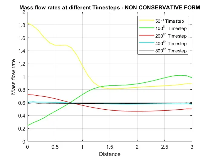
Mass flow rate at different timesteps:

1. Non-conservative form

2. Conservative form

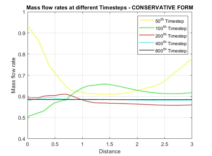
From the above plots of conservative and non-conservative form, I conclude that the solution is started converge to a stable solution after 400th iteration in both forms.

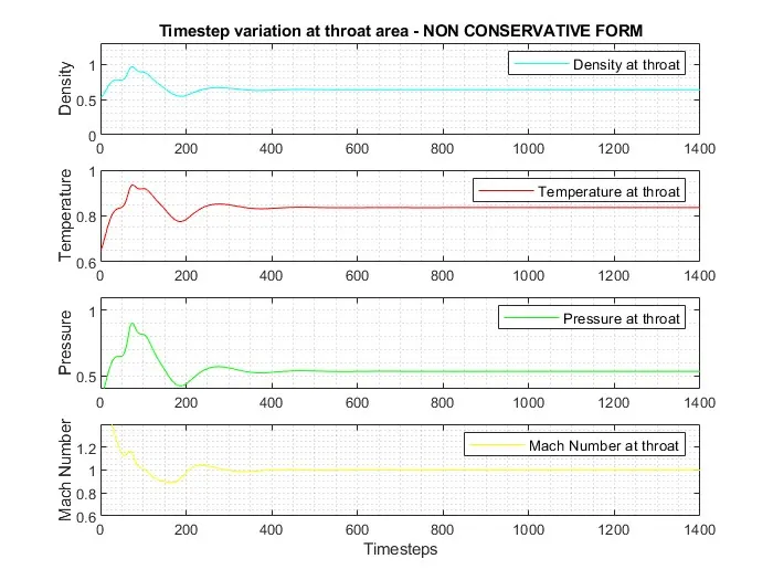
Timestep variation at throat area:

1. Non-conservative form

2. Conservative form

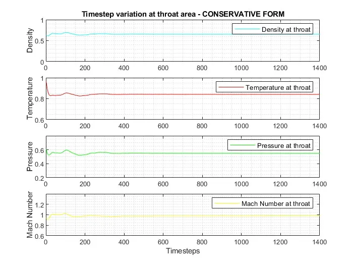
From the above plots of conservative and non-conservative form, I conclude that the conservative form achieves more stable solution after some period of time compared to non-conservative forms.

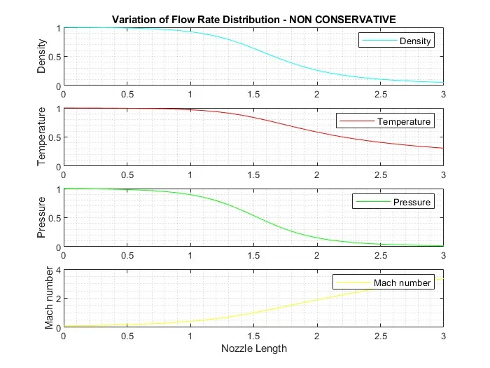
Variation of flow rate distribution:

1. Non-conservative form

2. Conservative form

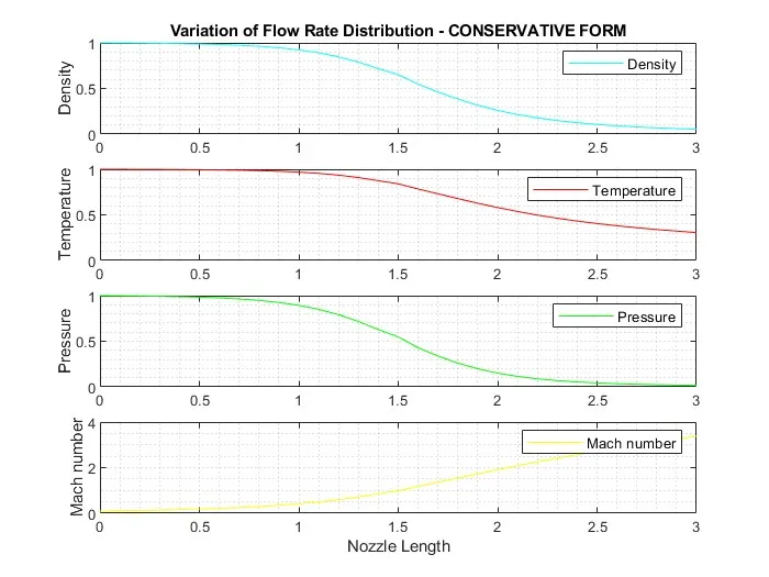
From the above plots of conservative and non-conservative form, I conclude that the both plots are same thus the variation of flow rate distribution through the nozzle is same.

Comparison of mass flow rate of both forms:

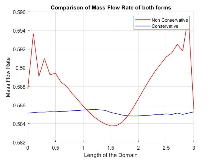
From the above plot, I conclude that the mass flow rate of conservative form is more stable compared to non-conservative form.

Comparison of solution values at final timestep with different number of node points:

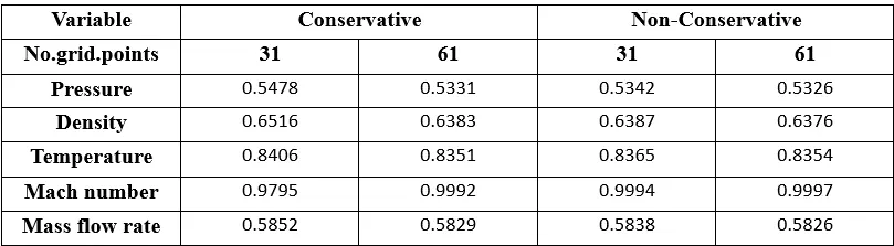
From above table, I observe that when increasing number of grid points there is a slight variation in the solution values. But it doesn't affect the solution values.

Conclusion:

From the results, I conclude that conservative form is more stable and converges faster compared to non-conservative form.
The mass flow rate of conservative form is more stable compared to non-conservative form.
Increasing the number of grid points doesn't have any significant effect in the solution results.

Week 7 - Simulation of a 1D Supersonic nozzle flow simulation using Macormack Method

SIMULATION OF A 1D-SUPERSONIC NOZZLE FLOW SIMULATION USING MACCORMACK METHOD

Ship work like this
in your own course.

Talk to a career counsellor

SIMULATION OF A 1D-SUPERSONIC NOZZLE FLOW SIMULATION USING MACCORMACK METHOD

Ship work like thisin your own course.

Talk to a career counsellor

Ship work like this
in your own course.