Week 7 - Simulation of a 1D Supersonic nozzle flow simulation using Macormack Method
Objective: simulate the isentropic flow through a quasi 1D subsonic-supersonic nozzle. You will derive both the conservation and non-conservation forms of the governing equations and sovle them using the MacCormack's technique.
Theory:
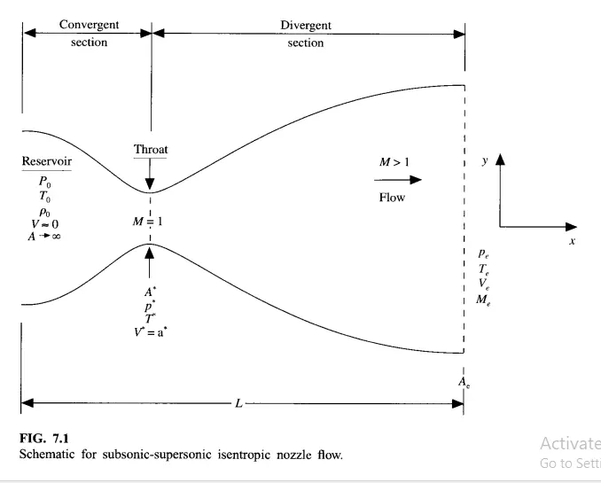
We consider the steady, isentropic flow through a convergent-divergent nozzleas sketched in Fig. 7.1. The flow at the inlet to the nozzle comes from a reservoirwhere the pressure and temperature are denoted by p_{0} , and T_{0} , respectively. Thecross-sectional area of the reservoir is large (theoretically, A -> ∞ ), and hence thevelocity is very small (V -> 0) . Thus, p_{0} and T_{0} are the stagnation values, or totalpressure and total temperature, respectively. The flow expands isentropically tosupersonic speeds at the nozzle exit, where the exit pressure, temperature, velocity,and Mach number are denoted by p_{e} T_{e} V_{o} and M_{e} respectively. The flow islocally subsonic in the convergent section of the nozzle, sonic at the throat(minimum area), and supersonic at the divergent section the local speed of the sound.
Quasi 1D:
In reality the flow was one dimentional but we make an assumption that the flow properties veryis along x axis. trantamount to assumuing that the uniform flow properties across any given crossection, such flow is defined as quasi-one-dimensional-flow.
Conservation from of equation:
continuty equation:
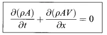
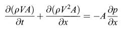
momentum equation:
Energy equaion:

Non-conservation from of equation:
In the one dimetional flow if we take aria as constand then the equation is called the non-conservation from of the equation. because the in this equation it doesnot define the mass flow rate properly, In practical way A=A(x).
Continuty equation:

Momentum Equaion:

Energy equation:

Now Non Dimetionalize the Non -conserved from of equation:
Non-Dimentional from of veriable are T'=T/T0,rho'=rho/rho0, x'=x/L,V'=v/a0,t'=t/(L/a0)
a0=root(gama*R*T0)
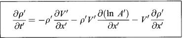
continuty equation is
Momentom Equation:
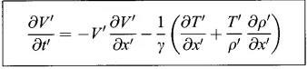
Energy Equation:

Mac-Cormak method to solve the Non_conventional from of equation:
Predicted step:
In this step we find the change of veriable with respect to time in present time:



Then we calculate the predicted step for next time step by useing the rate of change of present veriable.
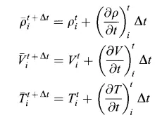
Corrected value of rate of change:
Then calculate the corrected value of rate of change of the veriable of next time step by useing the predicted value of next time step. here we do the backword differences.
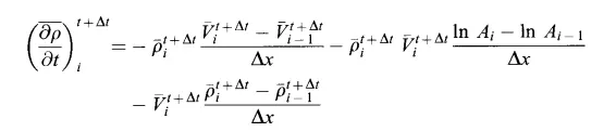

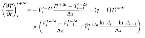
Now calculate the avaerage rate of change of the variable by useing the average of both predicted and corrected value.
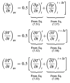
Then we calculate the values for the next time step by useing average time derivative of the veriable.
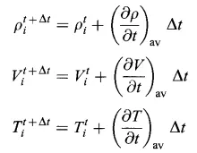
Find the time step value:
For stability of the solution we must follow the courent no,other wise the solution will unstable if we take very small dt value,if we take the very higher time step value then it is very defficalt to cover time marching proper way.
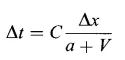
Here ΔX is same for all node but a and v both are function of x
now
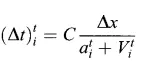
for adjacent node
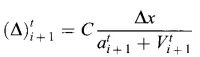
Now proper value of the Δt we have to find the value of the minmum of the Δt.

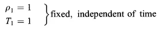
Initial condition:

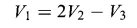
Boundery condition:
Matlab code for the Non_conservcative equation:
clear all
close all
clc
%input
n=31;
x=linspace(0,3,n);
dx=x(2)-x(1);
%calculate project profile
rho=1-0.3146*x;
t=1-0.2314*x;
v=(0.1+1.09*x).*t.^0.5;
a=1+2.2*(x-1.5).^2;
gama=1.4;
%plot(a)
%time step
nt=1400;
dt=0.01;
%For outer timeloop
for k=1:nt
rho_old=rho;
v_old=v;
t_old=t;
%for predicter method
for j=2:n-1
dvdx=(v(j+1)-v(j))/dx;
drhodx=(rho(j+1)-rho(j))/dx;
dtdx=(t(j+1)-t(j))/dx;
dlog_a_dx=(log(a(j+1))-log(a(j)))/dx;
%conyinuty equation
drhodt_p(j)=-rho(j)*dvdx-rho(j)*v(j)*dlog_a_dx-v(j)*drhodx;
%momentum equation
dvdt_p(j)=-v(j)*dvdx-(1/gama)*(dtdx+(t(j)/rho(j))*drhodx);
%energy equation
dtdt_p(j)=-v(j)*dtdx-(gama-1)*t(j)*(dvdx+v(j)*dlog_a_dx);
%solution update
rho(j)=rho(j)+drhodt_p(j)*dt;
v(j)=v(j)+dvdt_p(j)*dt;
t(j)=t(j)+dtdt_p(j)*dt;
end
%corrected method
for i=2:n-1
dvdx=(v(i)-v(i-1))/dx;
drhodx=(rho(i)-rho(i-1))/dx;
dtdx=(t(i)-t(i-1))/dx;
dlog_a_dx=(log(a(i))-log(a(i-1)))/dx;
%conyinuty equation
drhodt_c(i)=-rho(i)*dvdx-rho(i)*v(i)*dlog_a_dx-v(i)*drhodx;
%momentum equation
dvdt_c(i)=-v(i)*dvdx-(1/gama)*(dtdx+(t(i)/rho(i))*drhodx);
%energy equation
dtdt_c(i)=-v(i)*dtdx-(gama-1)*t(i)*(dvdx+v(i)*dlog_a_dx);
end
%compute avaerage time darivative
drhodt=0.5*(drhodt_p+drhodt_c);
dvdt=0.5*(dvdt_p+dvdt_c);
dtdt=0.5*(dtdt_p+dtdt_c);
%final solution update
for i=2:n-1
rho(i)=rho_old(i)+drhodt(i)*dt;
v(i)=v_old(i)+dvdt(i)*dt;
t(i)=t_old(i)+dtdt(i)*dt;
end
%boundery condition
%incial boundery condition
rho(1)=2*rho(2)-rho(3);
v(1)=2*v(2)-v(3);
t(1)=2*t(2)-t(3);
%final boundery
rho(n)=2*rho(n-1)-rho(n-2);
v(n)=2*v(n-1)-v(n-2);
t(n)=2*t(n-1)-t(n-2);
p=rho.*t;
pressure(k)=p(16);
dencity(k)=rho(16);
tempreture(k)=t(16);
m(k)=k;
figure(1)
plot(x,v)
xlabel('x')
ylabel('velocity')
figure(2)
plot(x,rho)
xlabel('x')
ylabel('dencity')
figure(3)
plot(x,t)
xlabel('x')
ylabel('tempreture')
figure(4)
plot(x,t)
xlabel('x')
ylabel('presurre')
plot(m,pressure)
xlabel('time step')
ylabel('presurre')
pause(0.03)
figure(6)
plot(m,dencity)
xlabel('time step')
ylabel('dencity')
figure(7)
plot(m,tempreture)
xlabel('time step')
ylabel('tempreture')
end
Output:
1.Steady-state distribution of primitive variables inside the nozzle:
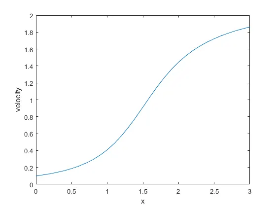
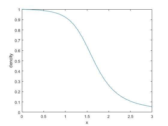
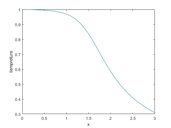
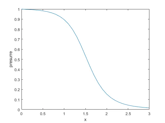
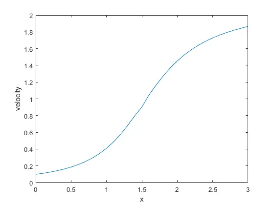
- Output velocity of the after stedy state is 1.8 time of the sound speed. From this plot we observe that in the convergre section there is sharp increase in the velocity,due to decrease in the aria.But in the divergent region velocity was not decresing .
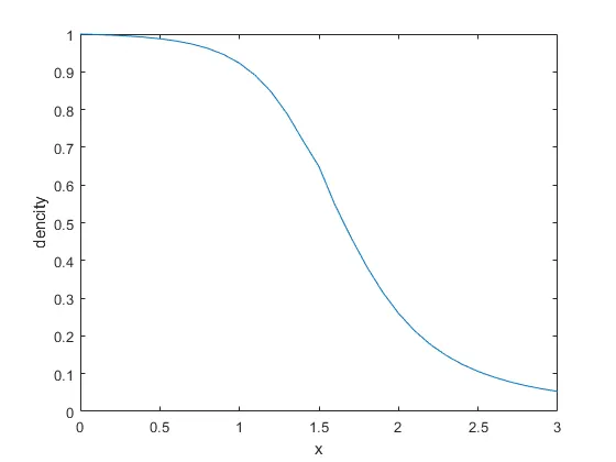
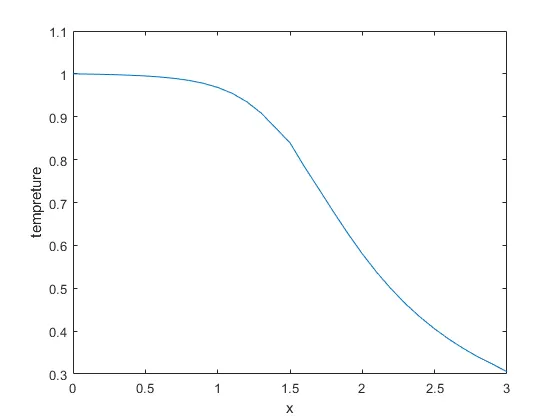
- Dencity,tempreture,pressure these properties are change with distence toward the outlet.
2. Time-wise variation of the primitive variables:
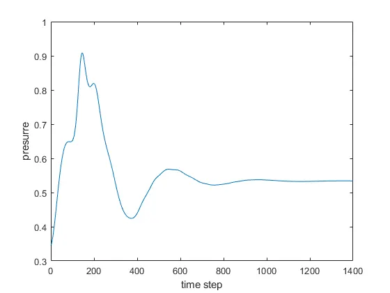
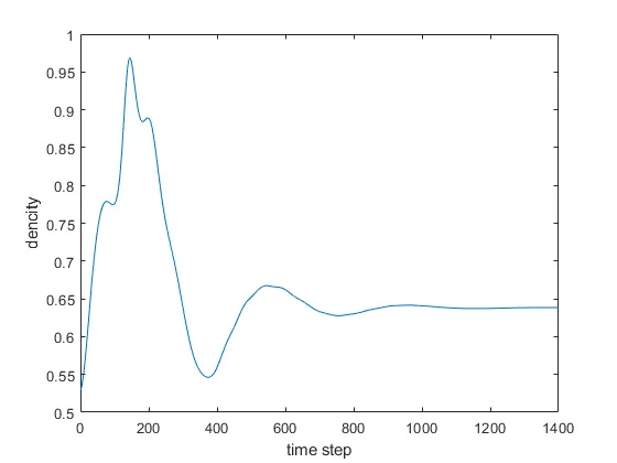
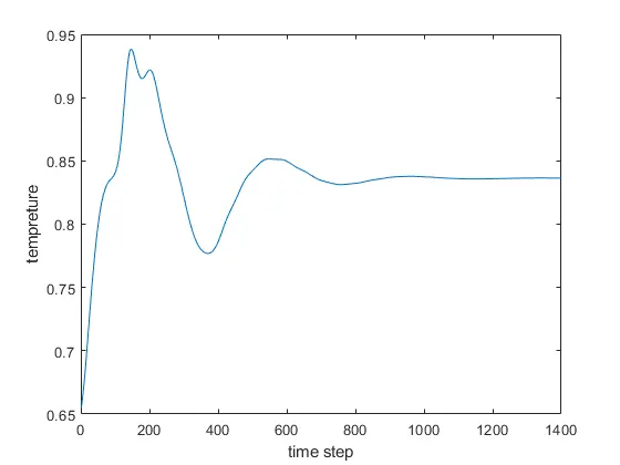
- Here incitaly the plots are start from Zero because it represent the incial condition, then in sharp manner the veriable are increseing,then become steady.this is called 'rouber band effect'.if we strached the rouber band then there is a high potencial. due to the igh potencial the veriables are change sharply then become stable.
- When veriable are stable, that represent bend was relaxed.
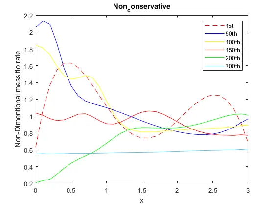
Variation of Mass flow rate distribution inside the nozzle at different time steps during the time-marching process:
Solution of the conservative from of equation:
Nondimational from of conservative equation
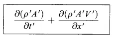
Continuty equation:
Momentum Equation:

Energy Equation:

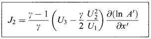
Let us define these equation by the U as solution veriable,F flux veriable,J as the source term.
Now defined as:
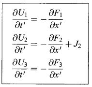
and
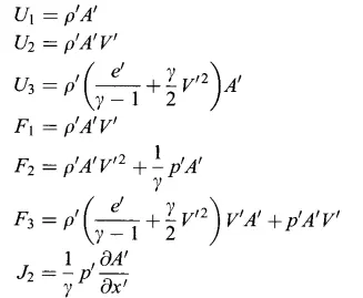
Now Convert flux term in to the solution term:

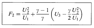
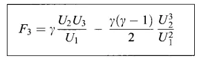
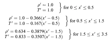
Initial Condition:
Boundery condition:
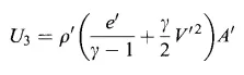
Inlet Boundery condition:


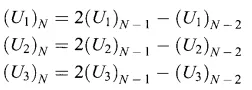
Outlet Boundery condition:
Matlab code for the Conservaive from:
clear all
close all
clc
%grid creatuon
n=31;
x=linspace(0,3,n);
dx=x(2)-x(1);
a=1+(2.2*((x-1.5).^2));
gama=1.4;
nt=1400;
for i=1:n
%incialize the value of veriable
if(x(i)<=0.5)
rho(i)=1;
t(i)=1;
v(i)=0.59/(rho(i)*a(i));
else if(x(i)>=0.5 && x(i)<=1.5 )
rho(i)=1-(0.366*(x(i)-0.5));
t(i)=1-(0.167*(x(i)-0.5));
v(i)=0.59/(rho(i)*a(i));
else
rho(i)=0.634-(0.3879*(x(i)-1.5));
t(i)=0.833-(0.3507*(x(i)-1.5));
v(i)=0.59/(rho(i)*a(i));
end
end
end
%solution veriable
u1=rho.*a;
u2=rho.*a.*v;
u3=rho.*a.*((t/(gama-1))+((gama/2)*v.^2));
p=rho.*t;
dt=0.0267;
for k=1:nt
f1=u2;
f2=((u2.^2)./u1)+(((gama-1)/gama)*(u3-((gama/2)*(u2.^2./u1))));
f3=((gama*u2.*u3)./u1)-((gama*(gama-1)/2)*((u2.^3)./(u1.^2)));
uold1=u1;
uold2=u2;
uold3=u3;
%compute predicted step
for j=2:n-1
J1(j)=(1/gama)*p(j)*((a(j+1)-a(j))/dx);
%find the time derivative
du1dt_p(j)=-(f1(j+1)-f1(j))/dx;
du2dt_p(j)=-((f2(j+1)-f2(j))/dx)+J1(j);
du3dt_p(j)=-(f3(j+1)-f3(j))/dx;
%find the predicted value of the present tine step
u1(j)=u1(j)+du1dt_p(j)*dt;
u2(j)=u2(j)+du2dt_p(j)*dt;
u3(j)=u3(j)+du3dt_p(j)*dt;
end
%compute the veriable
rho=u1./a;
v=u2./u1;
t=(gama-1)*((u3./u1)-(gama/2)*v.^2);
p=rho.*t;
f1=u2;
f2=((u2.^2)./u1)+(((gama-1)/gama)*(u3-((gama/2)*(u2.^2./u1))));
f3=((gama*u2.*u3)./u1)-((gama*(gama-1)/2)*(u2.^3./u1.^2));
%corrected step
for j=2:n-1
J1=(1/gama)*p(j)*(a(j)-a(j-1))/dx;
%find the time derivative
du1dt_c(j)=-(f1(j)-f1(j-1))/dx;
du2dt_c(j)=-((f2(j)-f2(j-1))/dx)+J1;
du3dt_c(j)=-(f3(j)-f3(j-1))/dx;
%find the predicted value of the present tine step
end
%average time derivative
du1dt_avg=0.5*(du1dt_c+du1dt_p);
du2dt_avg=0.5*(du2dt_c+du2dt_p);
du3dt_avg=0.5*(du3dt_c+du3dt_p);
%calculate solution veriable
for i=2:n-1
u1(i)=uold1(i)+du1dt_avg(i)*dt;
u2(i)=uold2(i)+du2dt_avg(i)*dt;
u3(i)=uold3(i)+du3dt_avg(i)*dt;
end
%susution update
%inlet boundery condition
u1(1)=rho(1)*a(1);
u2(1)=2*u2(2)-u2(3);
u3(1)=u1(1)*((t(1)/(gama-1))+((gama/2)*v(1)^2));
%outlet boundery condition
u1(n)=2*(u1(n-1))-u1(n-2);
u2(n)=2*(u2(n-1))-u2(n-2);
u3(n)=2*(u3(n-1))-u3(n-2);
rho=u1./a;
v=u2./u1;
t=(gama-1)*((u3./u1)-(gama/2)*v.^2);
p=rho.*t;
pressure(k)=p(16);
dencity(k)=rho(16);
tempreture(k)=t(16);
m(k)=k;
mass_flow_rate(:,k)=rho.*a.*v;
end
figure(1)
plot(x,v)
xlabel('x')
ylabel('velocity')
figure(2)
plot(x,rho)
xlabel('x')
ylabel('dencity')
figure(3)
plot(x,t)
xlabel('x')
ylabel('tempreture')
figure(4)
plot(x,p)
xlabel('x')
ylabel('presurre')
figure(5)
plot(m,pressure)
xlabel('time step')
ylabel('presurre')
pause(0.03)
figure(6)
plot(m,dencity)
xlabel('time step')
ylabel('dencity')
figure(7)
plot(m,tempreture)
xlabel('time step')
ylabel('tempreture')
figure(8)
grid on
plot(x,mass_flow_rate(:,1),'color','r','linestyle','--');
hold on
plot(x,mass_flow_rate(:,50),'color','blue')
plot(x,mass_flow_rate(:,100),'color','yello')
plot(x,mass_flow_rate(:,150),'color','r')
plot(x,mass_flow_rate(:,200),'color','green')
plot(x,mass_flow_rate(:,700))
legend('1st','50th','100th','150th','200th','700th');
Steady-state distribution of primitive variables inside the nozzle:
Time-wise variation of the primitive variables:
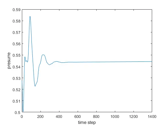
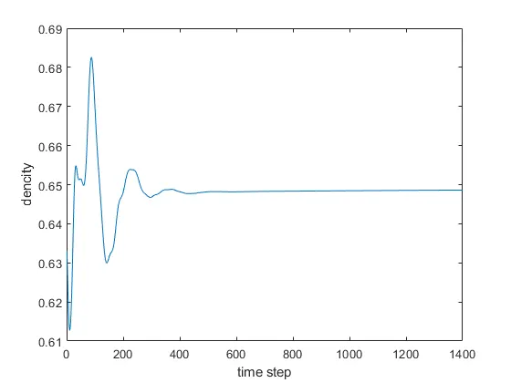
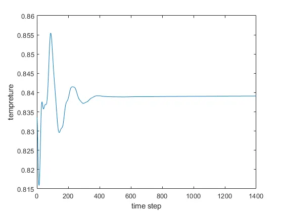
- In conservative from of equation the solution is not start from the zero,because we use the flax of premitive veriable other then premitive veriable .
- Here we need very less time step to converge to the stady state then the non-conservative from of Equation.
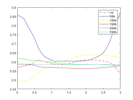
Variation of Mass flow rate distribution inside the nozzle at different time steps during the time-marching process:
Comparison of Normalized mass flow rate distributions of both forms:
- Now if we cnsider the first ittration ,we found incial massflow rate throgh out the nozzel of conservative flow is more unfrom then the non conservative flow.
- It is because of the representation of the premitive veriable,In the non-conservative process we found the veriable at the node point, which reprasent the whole section.But in the coservative from the primitive veriables are come from flux veriable which represent velue of per unit area.
- So initial non-conservative plot mass flow rate in biger is high.
- Now we look into the till 200 no of ittration we found mass flow rate was not stable.
- If we compear both the plot ,we found mass flow rate of coservative from is more stable then non-conservative, because it approching stable mass flow tate more faster in conservative equation.
- If we closely check the 700 itrration we found there is some unstability in mass flow rate still there in non-consevative flow. beacuse In non-coservative flow premitive veriables comes to steady with less no of ittration.
Conclusion:
- If we consider Outputs then we get conservative from of equation is prefered.
- But we take codeing and stability ascpect,Non-cosevative equation is preferable.In non-consevative from of equation primitive veriables can found directly, So it is eassy to code.
- In coservative equation first we found solution veriable from flux veriable then we found primitive veriable.so there is achence of increasing of error with every ittration.