Week 7 - Simulation of a 1D Supersonic nozzle flow simulation using Macormack Method

Aim: Stimulation of a one-dimensional super-sonic nozzle flow simulation using Maccormack method. 

Objective:

To simulate the isentropic flow through a quasi 1D subsonic-supersonic nozzle by deriving both the conservation and non-conservation forms of the governing equations and solving them using Maccormack's technique. And also determine the steady-state temperature distribution for the flow-field variables and investigate the difference between the two forms of governing equations by comparing their solutions, and plot the following:

• Steady-state distribution of primitive variables inside the nozzle.
• Time-wise variation of the primitive variables.
• Variation of Mass flow rate distribution inside the nozzle at different time steps during the time-marching process.
• Comparison of Normalized mass flow rate distributions of both forms.

Theory:

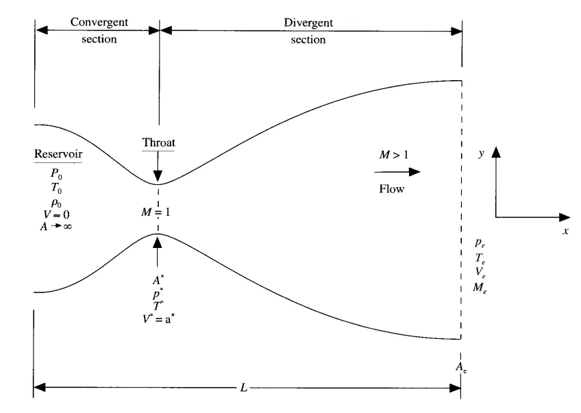
We consider the steady, isentropic flow through a convergent-divergent nozzle as sketched below. The flow at the inlet to the nozzle comes from a reservoir where the pressure and temperature are denoted by Po, and To, respectively. The cross-sectional area of the reservoir is large (theoretically, A→ ∞), and hence the velocity is very small (V → 0). Thus, po and to are the stagnation values, or total pressure and total temperature, respectively. The flow expands entropically to supersonic speeds at the nozzle exit, where the exit pressure, temperature, velocity, and Mach number are denoted by Pe, Te, Ve, and Me, respectively. The flow is locally subsonic in the convergent section of the nozzle, sonic at the throat (minimum area), and supersonic at the divergent section. The sonic flow (M = 1) at the throat means that the local velocity at this location is equal to the local speed of sound. Using an asterisk to denote sonic flow values, we have at the throat V = V* = a*. Similarly, the sonic flow values of pressure and temperature are denoted by p* and T*, respectively. The area of the sonic throat is denoted by A*. We assume that at a given section, where the cross-sectional area is A, the flow properties are uniform across that section. Hence, although the area of the nozzle changes as a function of distance along the nozzle, x, and therefore in reality the flow field is two-dimensional (the flow varies in the two-dimensional xy space), we make the assumption that the flow properties vary only with x; this is tantamount to assuming uniform flow properties across any given cross section. Such flow is defined as quasi-one-dimensional flow.

The governing flow equations will be couched in terms of partial differential equations suitable for the time-marching solution of quasi-one-dimensional flow using conservative or non-conservative equations. The continuity, momentum, and energy equations in the conservative and non-conservative form are given below.

Solving using non-Conservation method:

• Continuity equation:
  
• Momentum equation:
  
• Energy equation:
  

Here, we define the dimensionless length as  

Denoting the speed of sound in the reservoir as a₀, where
                   
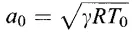
we define a dimensionless velocity as 

Also, the quantity L/a₀ has the dimension of time, and we define a dimensionless time as

Finally, we ratio the local area A to the sonic throat area A* and define a dimensionless area as
             

Maccormack's technique is a Predictor-Corrector method. First, consider the predictor step. Now, we set up the spatial derivatives as forward differences. Also, to reduce the complexity of the notation, we will drop the use of the prime to denote a dimensionless variable. In what follows, all variables are the nondimensional variables, denoted earlier by the prime notation. 

Continuity Equation:

Momentum Equation:

Energy Equation:

The predicted parameters values like ρ, V and T are 

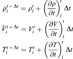
Then moving to Corrector step:

Continuity Equation:

Momentum Equation:

Energy Equation:

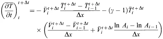
Then, the average Time derivatives are given by 

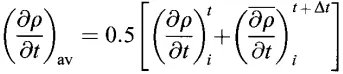
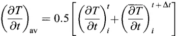
Boundary conditions:

Subsonic inflow boundary conditions:

Supersonic outflow boundary conditions:

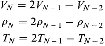
Initial conditions:  At t = 0

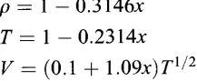
Nozzle shape: The nozzle shape, A = A(x), is specified and held fixed, independent of time.

Solving using Conservation method:

The equations in Conservation form are 

Continuity Equation:

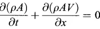
Momentum equation:

.

Energy Equation:

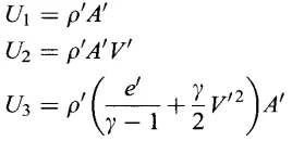
Let us define the elements of the solutions vector U, the flux vector F, and the source term J as follows.

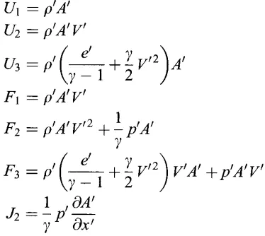
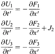
Then, the non-dimensional conservation form equations are written as 

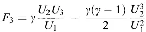
To setup the numerical solution at each time step by writing the F1, F2, F3, J2 in term of U1, U2, U3 is

Boundary conditions:

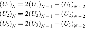
The boundary conditions for the subsonic-supersonic isentropic flow solution using the conservation form of the governing equations are the same. And also

Initial conditions:

Matlab code:

main code

For conservation form

For Non-Conservation form

Explanation:

• In the main code first, defined the input parameters of the problem like x, dx, n, gamma, c, L, nt.
• Then, defined the non-conservation and conservation form functions that are mentioned separately with required details.
• In the conservation form function, we written the initial conditions of density, temperature, velocity, area, Mach number and mass flow rate. Then created the time loop, then defined the Predicted method by writing the continuity, momentum, and energy equations and at the end of the predicted method update the solution terms.
• Then defined the corrected term loop by writing the spatial term equations of continuity, momentum and energy terms. 
• Then calculated the average of predictive and corrective methods and termed it as average time derivative. And update the old solution terms.
• Then, mention both subsonic and supersonic boundary conditions. Then define the final solution terms.
• Then, calculate solution term values inside the nozzle that means at the throat point where, throat =((n-1)/2) +1 = 16.
• Then, plot the graphs of mass flow rate at different timesteps, Steady-state distribution of primitive variables, Time-wise variation of the primitive variables at throat point.
• Now, coming to the non-conservation form function, the initial boundary conditions differ from the previous function, and here we define the initial solution vectors U1, U2, U3. Then determined the time step variable dt, and the remaining initial conditions of solution terms.
• Then, updated the initial solution vectors at the end of the loop. Then defined the Flux vectors F1, F2, F3. Then calculated the Predicted method terms and updated the solution vectors and primitive terms and Flux vectors at the end of the loop.
• Then, we calculated the corrective method terms and then calculated the average time derivatives by averaging the predictive and corrective terms. After that define the final boundary conditions, and update the final primitive terms.
• Then, calculate the primitive term values at the point of throat, then plot the mass flow rate at different timesteps, Steady-state distribution of primitive variables, and Time-wise variation of the primitive variables at throat point.
• And in the main code plot the figures of Mass flow rate using "non-Conservative form vs Conservative form" at throat point, and Conservative form and Non conservation form: Grid independence test at throat point and Steady state simulation for primitive values for both non-Conservative form and Conservative form.
   

Results:

conservative form

Figure 1.

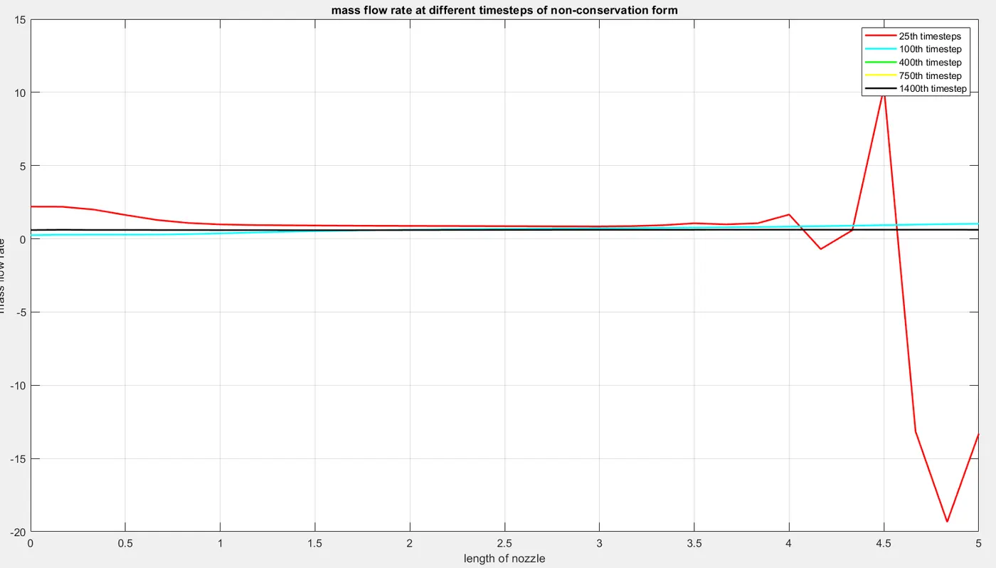
Figure 2.

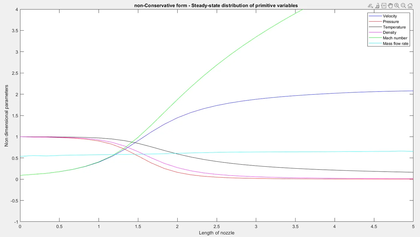
Figure 3.

Observations:

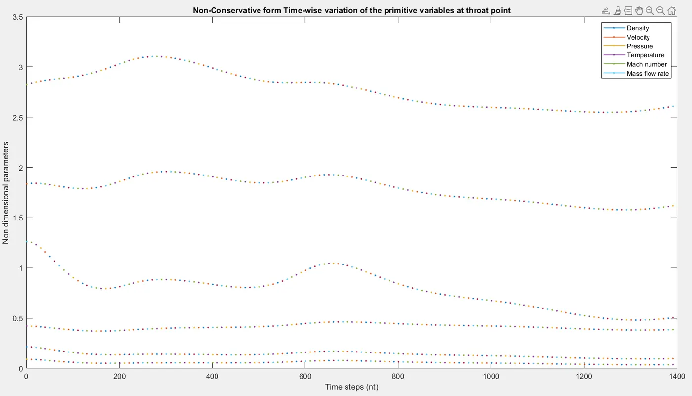
By increasing the nozzle length, the math number and velocity parameters increase and the density, mass flow rate, density terms are decreased. And the mass flow rate terms at different timesteps and at increasing rate of nozzle length gets increases up to a short length of nozzle then decreases.  And in the time wise variation of primitives the variables consumed high time to stabilize.

Figure 4.

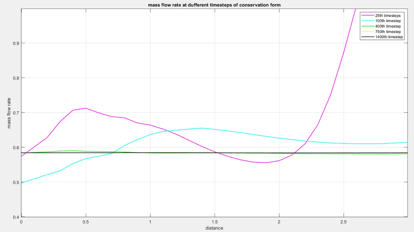
Figure 5.

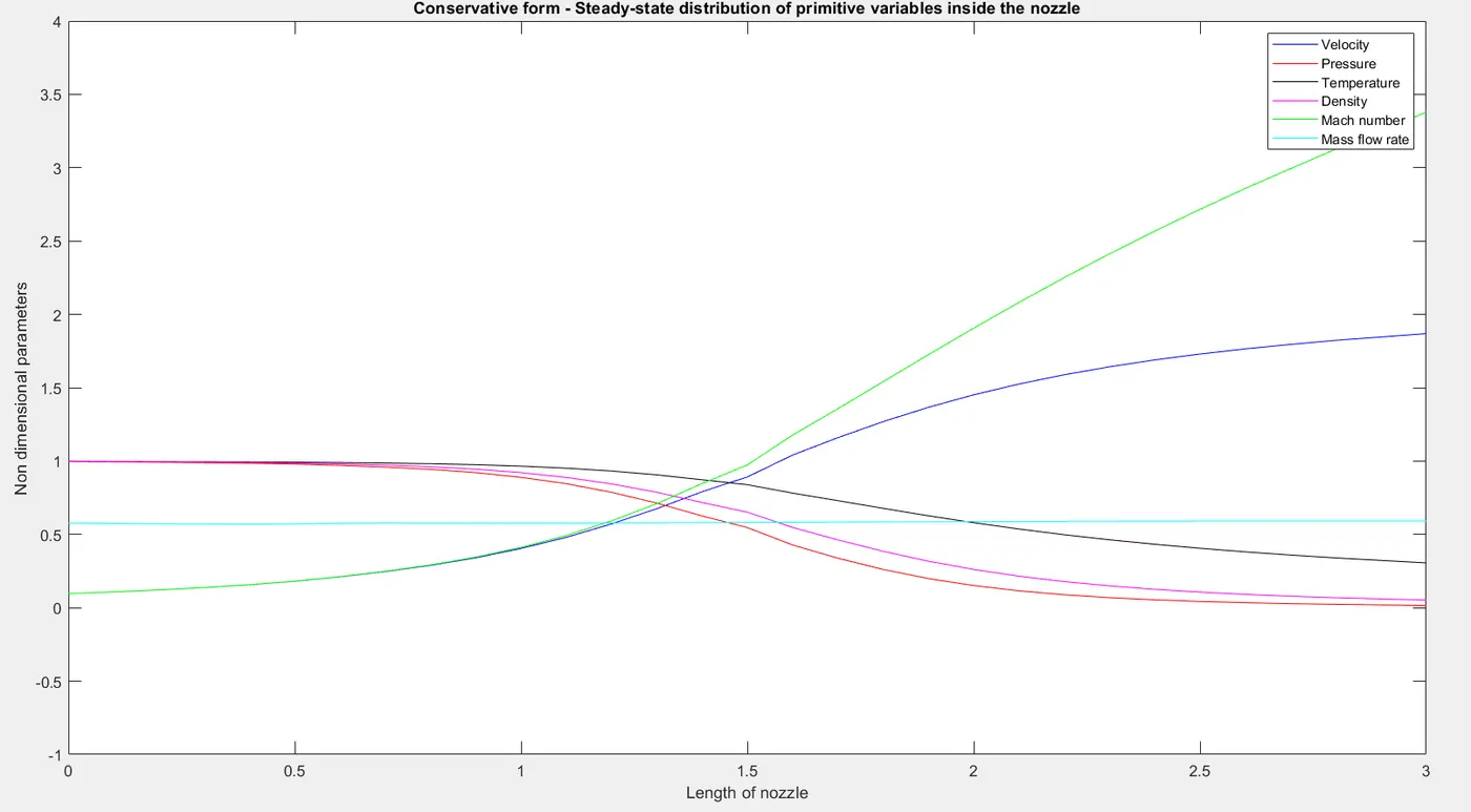
Figure 6.

Observations:

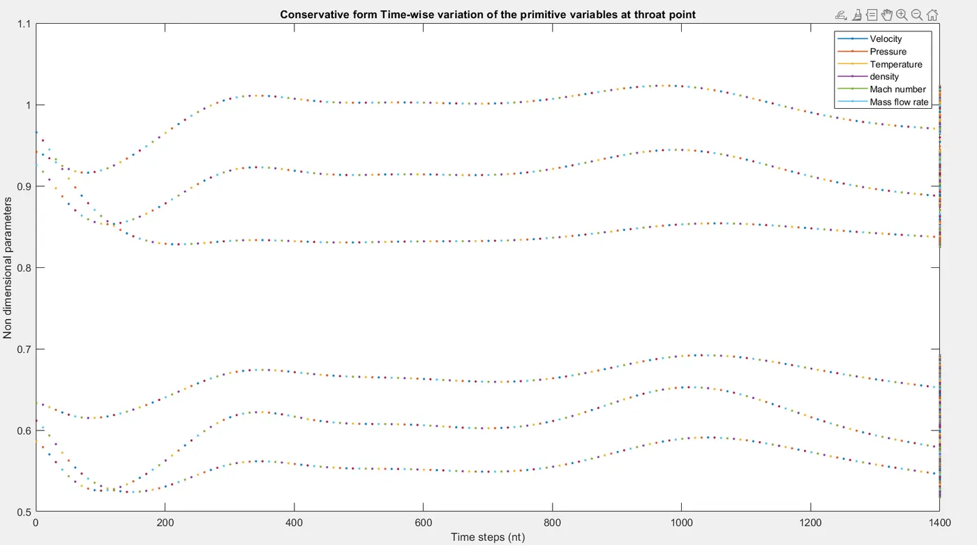
The mass flow rate term acts stable at timestep greater than 400 with respect to high nozzle length and the non-dimensional parameters consumed less time to become stable and almost same at the point of throat

Figure 7.

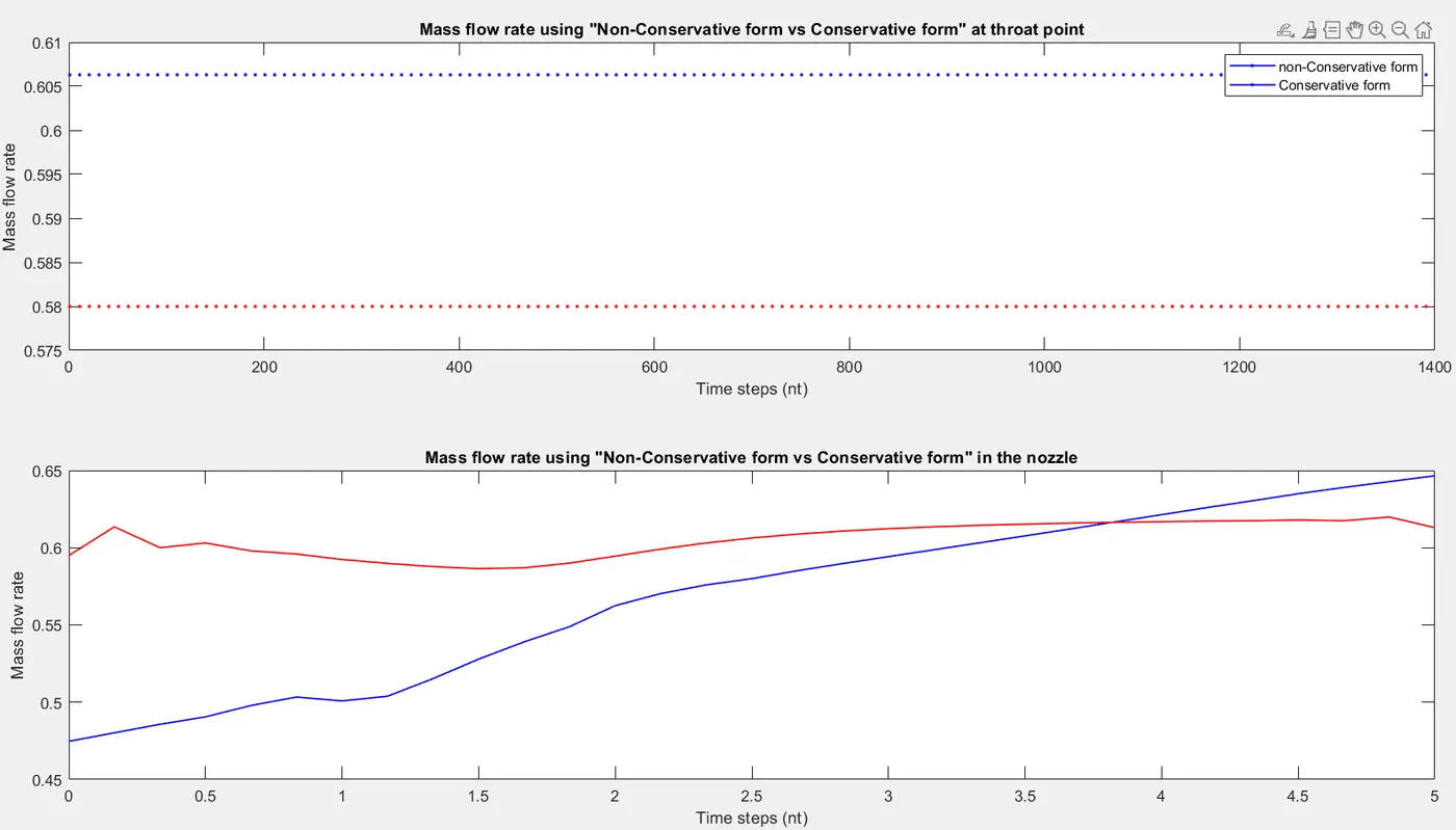
observation:

in the subplot 1 the both forms plots are similar and stable at every timestep. And in subplot 2 the conservative form plots are stable gradually increased with respect to timestep, and the non-conservative plots are almost stable at every timestep.

Figure 8.

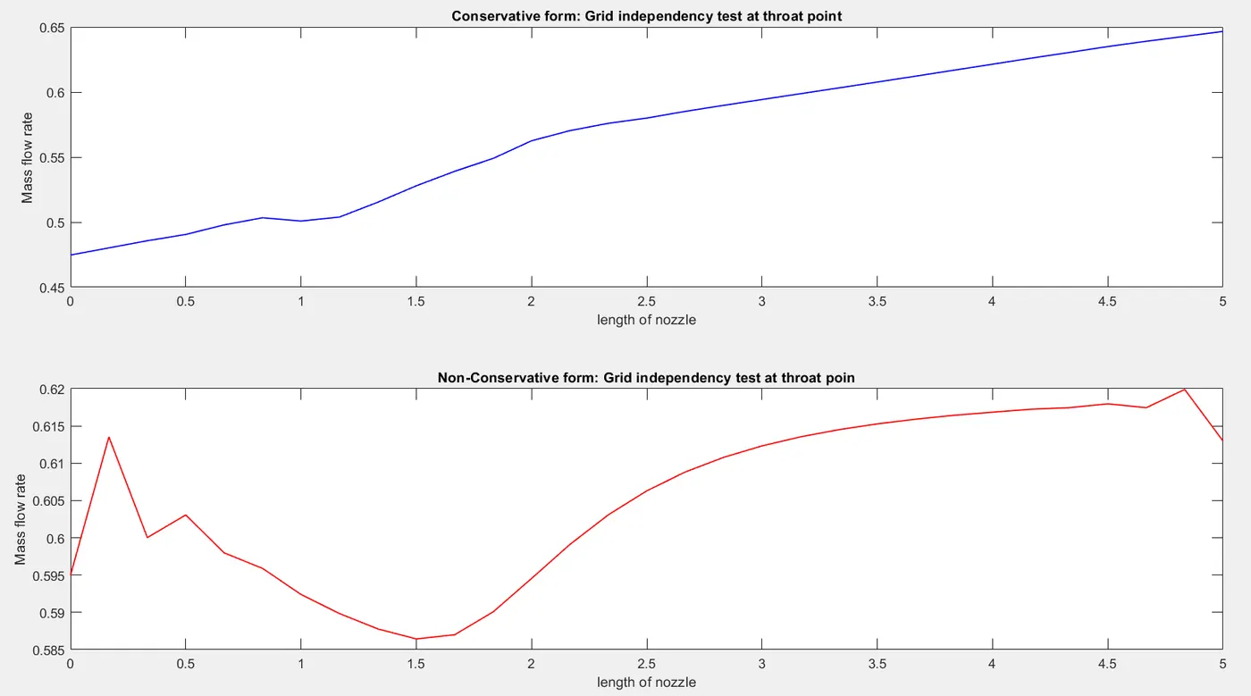
Observations:

The mass flow rate at throat point of non-conservative form is high at short length of nozzle and decreases up to a length of 1.5 then increases. And the mass flow rate at the throat point of conservative form increases with respect to increase of length of nozzle.

Figure 9.

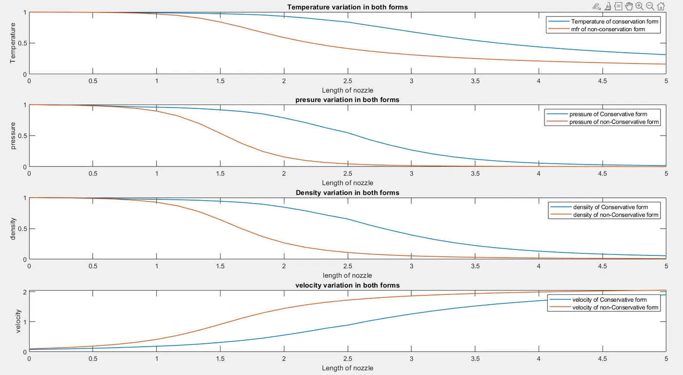
Here the nondimensional variables are plotted in both conservative and non-conservative forms with respect to nozzles length, here the Temperature gradually decrease in both the forms and the pressure variant high at minimum nozzle length and decreases with respect to increase of nozzle length. And the density term is similar to pressure variant and the velocity term gradually increases w.r.t to nozzle length.