Challenge

Week 7 - Simulation of a 1D Supersonic nozzle flow simulation using Macormack Method

SSaif Ansari1 Aug 2023

Aim : To simulate the isentropic flow through a quasi 1D subsonic-supersonic nozzle using the MacCormack's technique for conservation and non-conservation forms of the governing equations.

Introduction :

Converging-Diverging Nozzle is extensively used in a wide range of industrial applications ranging from steam turbines to rocket engine nozzles.
Here, we are achieving Supersonic Flows with Mach Number = 1 at the throat regions.It is also known as Choked Flow
As the fluid keeps on expanding at the diverging section of the nozzle, the fluid flow increases to achieve supersonic velocities with Mach Number > 1
If the choke conditions are not met, The Nozzle would simply act as Venturi Tube and would produce subsonic flow even the outlet
Mac-Cormack's Method is a variation of Lax-Wendroff Approach in which the latter's complex second order derivative is replaced by forward differences on the predictor and reward differences on the corrector
Mac-Cormack's Method is well suited for non-linear equations which is frequently encountered in our fluid-flow applications.

Governing Equations :

The Fluid Flow through the Nozzle is governed my continuity,momentum & energy equations.
The Flow is assumed to be Quasi-1d Flows,the conventional flows are slightly modified.

→ Continuity Equation

→ Momentum Equation

→ Energy Equation

Predictor And Corrector Method :

Here we are splitting Time Marching Method into Predictor & Corrector Method

Initial Condition - The initial condition for all the flow field variables are to be determined
Predictor Step - In this step, we are performing Forward Differencing Method

Solution Update - After Predictor Step, the initial values are updated

Corrector Step - In this step, we are performing Backward Differencing Method

Average Derivative - In this step, the average of predictor and Corrector are determined

Final Solution Update - Final Solution of the flow field variables are determined

Main Matlab Code

clear all

close all

clc

%% Inputs

disp("Enter the number of nodes")

n = input("nodes = "); %% Node = 31,61

gamma = 1.4;

x = linspace(0,3,n);

dx = x(2) - x(1);

%% No. of time step

nt = 1400;

%% Courant Number

C = 0.5;

%% Non Conservative Form

tic;

[Mass_Flow_Rate_NC, Pressure_NC, Mach_Number_NC, Rho_NC, V_NC, T_NC, Rho_Throat_NC, V_Throat_NC, T_Throat_NC, Mass_Flow_Rate_Throat_NC, Pressure_Throat_NC, Mach_Number_Throat_NC] = Non_conservative_form(x, dx, n, gamma, nt, C);

Time_Elasped_For_Non_Conservative_Form = toc;

%hold on

%% plot

%% Timestep variation of properties at throat area in Non Conservative form

figure(3)

%�nsity

subplot(4,1,1)

plot(linspace(1,nt,nt),Rho_Throat_NC,'color','#941d50',"LineWidth",2)

xlabel("TimeSteps","FontSize",10,"FontName","Times New Roman")

ylabel("Density Value","FontSize",9,"FontName","SansSerif")

legend("Density Throat Value V/S TimeSteps","FontSize",9,"FontName","Cambria");

axis([0 1400 0 1.3]);

title("Time Steps Variation For Non Conservative Form At Throat","FontSize",9,"FontName","Cambria");

%% Temperature

subplot(4,1,2)

plot(linspace(1,nt,nt),T_Throat_NC,'color','#947103',"LineWidth",2)

xlabel("TimeSteps","FontSize",10,"FontName","Times New Roman")

ylabel("Temeprature Value","FontSize",9,"FontName","SansSerif")

legend("Temperature Throat Value V/S TimeStep","FontSize",9,"FontName","Cambria");

axis([0 1400 0.6 1]);

%% Pressure

subplot(4,1,3)

plot(linspace(1,nt,nt),Pressure_Throat_NC,'color','#28059D',"LineWidth",2)

xlabel("TimeSteps","FontSize",10,"FontName","Times New Roman")

ylabel("Pressure Value","FontSize",9,"FontName","SansSerif")

legend("Pressure Throat Value V/S TimeStep","FontSize",9,"FontName","Cambria");

axis([0 1400 0.4 1.1]);

%% Mach Number

subplot(4,1,4)

plot(linspace(1,nt,nt),Mach_Number_Throat_NC,'color','#447202',"linewidth",2)

xlabel("TimeSteps","FontSize",10,"FontName","Times New Roman")

ylabel("Mach Number","FontSize",9,"FontName","SansSerif")

legend("Mach Number V/S TimeStep","FontSize",9,"FontName","Cambria");

axis([0 1400 0.6 1.4]);

%% Steady state simulation for primitve values for Non Conservative form

figure(4);

%�nsity

subplot(4,1,1);

plot(x,Rho_NC,'color','#941d50',"LineWidth",2)

xlabel("Nozzle Length","FontSize",10,"FontName","Times New Roman")

ylabel("Density Value","FontSize",9,"FontName","SansSerif")

legend("Density Value V/S Nozzle Length","FontSize",9,"FontName","Cambria");

axis([0 3 0 1])

title("Steady State Simulations For Non Conservative Form","FontSize",9,"FontName","Cambria")

%% Temperature

subplot(4,1,2);

plot(x,T_NC,'color','#947103',"LineWidth",2)

xlabel("Nozzle Length","FontSize",10,"FontName","Times New Roman")

ylabel("Temeprature Value","FontSize",9,"FontName","SansSerif")

legend("Temperature Value V/S Nozzle Length","FontSize",9,"FontName","Cambria");

axis([0 3 0 1])

%% Pressure

subplot(4,1,3);

plot(x,Pressure_NC,'color','#28059D',"LineWidth",2)

xlabel("Nozzle Length","FontSize",10,"FontName","Times New Roman")

ylabel("Pressure Value","FontSize",9,"FontName","SansSerif")

legend("Pressure Value V/S Nozzle Length","FontSize",9,"FontName","Cambria");

axis([0 3 0 1])

%% Mach number

subplot(4,1,4);

plot(x,Mach_Number_NC,'color','#447202',"linewidth",2)

xlabel("Nozzle Length","FontSize",10,"FontName","Times New Roman")

ylabel("Mach Number","FontSize",9,"FontName","SansSerif")

legend("Mach Number V/S Nozzle Length","FontSize",9,"FontName","Cambria");

axis([0 3 0 4])

%% conservative form function

tic;

[Mass_Flow_Rate_C, Pressure_C, Mach_Number_C, Rho_C, V_C, T_C, Rho_Throat_C, V_Throat_C, T_Throat_C, Mass_Flow_Rate_Throat_C, Pressure_Throat_C, Mach_Number_Throat_C] = Conservative_form(x, dx, n, gamma, nt, C);

Time_Elasped_For_Conservative_Form = toc;

%% Plotting

%% Timestep variation of properties at throat area in Conservative form

figure(5)

%�nsity

subplot(4,1,1)

plot(Rho_Throat_C,'color','#941d50',"LineWidth",2)

xlabel("TimeSteps","FontSize",10,"FontName","Times New Roman")

ylabel("Density Value","FontSize",9,"FontName","SansSerif")

legend("Density Throat Value V/S TimeSteps","FontSize",9,"FontName","Cambria");

axis([0 1400 0 1]);

title("Time Steps Variation For Conservative Form At Throat","FontSize",9,"FontName","Cambria")

%% Temperature

subplot(4,1,2)

plot(T_Throat_C,'color','#947103',"LineWidth",2)

xlabel("TimeSteps","FontSize",10,"FontName","Times New Roman")

ylabel("Temeprature Value","FontSize",9,"FontName","SansSerif")

legend("Temperature Throat Value V/S TimeSteps","FontSize",9,"FontName","Cambria");

axis([0 1400 0.6 1]);

%% Pressure

subplot(4,1,3)

plot(Pressure_Throat_C,'color','#28059D',"LineWidth",2)

xlabel("TimeSteps","FontSize",10,"FontName","Times New Roman")

ylabel("Pressure Value","FontSize",9,"FontName","SansSerif")

legend("Pressure Throat Value V/S TimeSteps","FontSize",9,"FontName","Cambria");

axis([0 1400 0.2 0.8]);

%% Mach Number

subplot(4,1,4)

plot(Mach_Number_Throat_C,'color','#447202',"linewidth",2)

xlabel("TimeSteps","FontSize",10,"FontName","Times New Roman")

ylabel("Mach Number","FontSize",9,"FontName","SansSerif")

legend("Mach Number Value V/S TimeSteps","FontSize",9,"FontName","Cambria");

axis([0 1400 0.6 1.4]);

%% Steady state simulation for primitve values for Conservative form

figure(6);

%�nsity

subplot(4,1,1);

plot(x,Rho_C,'color','#941d50',"LineWidth",2)

xlabel("Nozzle Length","FontSize",10,"FontName","Times New Roman")

ylabel("Density Value","FontSize",9,"FontName","SansSerif")

legend("Density Value V/S Nozzle Length","FontSize",9,"FontName","Cambria");

axis([0 3 0 1])

title("Steady State Simulations For Conservative Form","FontSize",9,"FontName","Cambria")

%% Temperature

subplot(4,1,2);

plot(x,T_C,'color','#947103',"LineWidth",2)

xlabel("Nozzle Length","FontSize",10,"FontName","Times New Roman")

ylabel("Temperature Value","FontSize",9,"FontName","SansSerif")

legend("Temperature Value V/S Nozzle Length","FontSize",9,"FontName","Cambria");

axis([0 3 0 1])

%% Pressure

subplot(4,1,3);

plot(x,Pressure_C,'color','#28059D',"LineWidth",2)

xlabel("Nozzle Length","FontSize",10,"FontName","Times New Roman")

ylabel("Pressure Value","FontSize",9,"FontName","SansSerif")

legend("Pressure Value V/S Nozzle Length","FontSize",9,"FontName","Cambria");

axis([0 3 0 1])

%% Mach number

subplot(4,1,4);

plot(x,Mach_Number_C,'color','#447202',"linewidth",2)

xlabel("Nozzle Length","FontSize",10,"FontName","Times New Roman")

ylabel("Mach Number","FontSize",9,"FontName","SansSerif")

legend("Mach Number V/S Nozzle Length","FontSize",9,"FontName","Cambria");

axis([0 3 0 4])

%% Mass Flow Rate Comparision

figure(7)

plot(x,Mass_Flow_Rate_NC,'color','#447202',"linewidth",2)

hold on;

plot(x,Mass_Flow_Rate_C,'color','#28059D',"linewidth",2)

legend("Non Conservative Form","Conservative Form","FontSize",9,"FontName","Cambria");

xlabel("Domain Length","FontSize",9,"FontName","SansSerif")

ylabel("Mass Flow Rate","FontSize",9,"FontName","SansSerif")

title("Comparision Of Mass Flow Rate For Conservative & Non Conservative Forms","FontSize",9,"FontName","Cambria")

Function Code For Non Conservative Method

function [Mass_Flow_Rate_NC, Pressure_NC, Mach_Number_NC, Rho_NC, V_NC, T_NC, Rho_Throat_NC, V_Throat_NC, T_Throat_NC, Mass_Flow_Rate_Throat_NC, Pressure_Throat_NC, Mach_Number_Throat_NC] = Non_conservative_form(x, dx, n, gamma, nt, C)

<!-- [if mso]>
<![endif]-->

%% Defining Initial Conditions

Rho_NC = 1 - 0.3146*x;

T_NC = 1 - 0.2341*x;

V_NC = (0.1 + 1.09*x).*T_NC.^0.5;

%% Defining Area & Throat Profiles

A = 1 + 2.2*(x-1.5).^2;

throat = find(A==1);

%% Outer Time Loop

for k = 1:nt

%% Time-Step

dt = min(C.*dx./(sqrt(T_NC) + V_NC));

%% Saving Old Values

rho_old = Rho_NC;

T_old = T_NC;

v_old = V_NC;

%% Predictor Method

for j = 2:n-1

%% Spatial Terms

dv_dx = (V_NC(j + 1) - V_NC(j))/dx;

drho_dx = (Rho_NC(j + 1) - Rho_NC(j))/dx;

dT_dx = (T_NC(j + 1) - T_NC(j))/dx;

dlog_a_dx = (log(A(j + 1)) - log(A(j)))/dx;

%% Continuity Equation

drho_dt_P(j) = -Rho_NC(j)*dv_dx - Rho_NC(j)*V_NC(j)*dlog_a_dx - V_NC(j)*drho_dx;

%% Momentum Equation

dv_dt_P(j) = -V_NC(j)*dv_dx - (1/gamma)*(dT_dx + (T_NC(j)*drho_dx/Rho_NC(j)));

%% Energy Equation

dT_dt_P(j) = -V_NC(j)*dT_dx - (gamma - 1)*T_NC(j)*(dv_dx + V_NC(j)*dlog_a_dx);

%% Solution Updation

Rho_NC(j) = Rho_NC(j) + drho_dt_P(j)*dt;

V_NC(j) = V_NC(j) + dv_dt_P(j)*dt;

T_NC(j) = T_NC(j) + dT_dt_P(j)*dt;

end

%% Corrector Method

for j = 2:n-1

%% Spatial Terms

dv_dx = (V_NC(j) - V_NC(j - 1))/dx;

drho_dx = (Rho_NC(j) - Rho_NC(j - 1))/dx;

dT_dx = (T_NC(j) - T_NC(j - 1))/dx;

dlog_a_dx = (log(A(j)) - log(A(j - 1)))/dx;

%% Continuity Equation

drho_dt_C(j) = - Rho_NC(j)*dv_dx - Rho_NC(j)*V_NC(j)*dlog_a_dx - V_NC(j)*drho_dx;

%% Momentum Equation

dv_dt_C(j) = - V_NC(j)*dv_dx - (1/gamma)*(dT_dx + (T_NC(j)*drho_dx/Rho_NC(j)));

%% Energy Equation

dT_dt_C(j) = - V_NC(j)*dT_dx - (gamma - 1)*T_NC(j)*(dv_dx + V_NC(j)*dlog_a_dx);

end

%% Average Time derivative

drho_dt = 0.5.*(drho_dt_P + drho_dt_C);

dv_dt = 0.5.*(dv_dt_P + dv_dt_C);

dT_dt = 0.5.*(dT_dt_P + dT_dt_C);

%% Final Solution Update

for i = 2:n-1

Rho_NC(i) = rho_old(i) + drho_dt(i)*dt;

V_NC(i) = v_old(i) + dv_dt(i)*dt;

T_NC(i) = T_old(i) + dT_dt(i)*dt;

end

%% Applying Boundary Conditions

%% At Inlet

Rho_NC(1) = 1;

V_NC(1) = 2*V_NC(2) - V_NC(3);

T_NC(1) = 1;

%% At Outlet

Rho_NC(n) = 2*Rho_NC(n-1) - Rho_NC(n - 2);

V_NC(n) = 2*V_NC(n - 1) - V_NC(n - 2);

T_NC(n) = 2*T_NC(n - 1) - T_NC(n - 2);

%�fining Mass Flow Rate, Pressure and Mach Number

Mass_Flow_Rate_NC = Rho_NC.*A.*V_NC;

Pressure_NC = Rho_NC.*T_NC;

Mach_Number_NC = (V_NC./sqrt(T_NC));

%�lculating Variables At Throat Section

Rho_Throat_NC(k) = Rho_NC(throat);

T_Throat_NC(k) = T_NC(throat);

V_Throat_NC(k) = V_NC(throat);

Mass_Flow_Rate_Throat_NC(k) = Mass_Flow_Rate_NC(throat);

Pressure_Throat_NC(k) = Pressure_NC(throat);

Mach_Number_Throat_NC(k) = Mach_Number_NC(throat);

%% Plotting

%% Comparison Of Non-Dimensional Mass Flow Rates At Different Time Steps

figure(1);

if k == 50

plot(x, Mass_Flow_Rate_NC,'color','#05B7CB',"LineWidth",1);

hold on

elseif k == 100

plot(x, Mass_Flow_Rate_NC,'color','#80026B ',"LineWidth",1 );

hold on

elseif k == 200

plot(x, Mass_Flow_Rate_NC,'color','#023180',"LineWidth",1);

hold on

elseif k == 400

plot(x, Mass_Flow_Rate_NC,'color','#027A80',"LineWidth",1 );

hold on

elseif k ==700

plot(x, Mass_Flow_Rate_NC,'color','#A69203',"LineWidth",1);

end

%% Labelling

title("Variation Of Mass Flow Rate At Different Time Steps For Non Conservative Form","FontSize",9,"FontName","Cambria")

xlabel('Distance',"FontSize",10,"FontName","Times New Roman")

ylabel('Mass Flow Rate',"FontSize",10,"FontName","SansSerif")

legend('50^t^h TimeStep','100^t^h TimeStep','200^t^h TimeStep','400^t^h TimeStep','700^t^h TimeStep',"FontSize",8,"FontName","Cambria")

axis([0 3 0 2])

end

Function Code For Conservative Method

function [Mass_Flow_Rate_C, Pressure_C, Mach_Number_C, Rho_C, V_C, T_C, Rho_Throat_C, V_Throat_C, T_Throat_C, Mass_Flow_Rate_Throat_C, Pressure_Throat_C, Mach_Number_Throat_C] = Conservative_form(x, dx, n, gamma, nt, C)

<!-- [if mso]>
<![endif]-->

%�fining Initial Conditions

for i = 1:n

if (x(i) >= 0 && x(i) <= 0.5)

Rho_C(i) = 1;

T_C(i) = 1;

elseif (x(i) >= 0.5 && x(i) <= 1.5)

Rho_C(i) = 1 - 0.366*(x(i) - 0.5);

T_C(i) = 1 - 0.167*(x(i) - 0.5);

elseif (x(i) >= 1.5 && x(i) <= 3)

Rho_C(i) = 0.634 - 0.3879*(x(i) - 1.5);

T_C(i) = 0.833 - 0.3507*(x(i) - 1.5);

end

%% Area & Throat profiles

A = 1 + 2.2*(x - 1.5).^2;

throat = find(A==1);

%% Initial profile fot Velocity and Pressure

V_C = 0.59./(Rho_C.*A);

Pressure_C = Rho_C.*T_C;

%�lculate the Initial Solution Vectors(U)

U1 = Rho_C.*A;

U2 = Rho_C.*A.*V_C;

U3 = Rho_C.*A.*(T_C./(gamma - 1)) + ((gamma/2).*V_C.^2);

%% Outer Time Loop

for k =1:nt

%% Time-step control

dt = min(C.*dx./(sqrt(T_C) + V_C));

%% Saving Old Values

U1_old = U1;

U2_old = U2;

U3_old = U3;

%�lculating the Flux vector(F)

F1 = U2;

F2 = ((U2.^2)./U1) + ((gamma - 1)/gamma)*(U3 - (gamma/2)*((U2.^2)./U1));

F3 = ((gamma*U2.*U3)./U1) - (gamma*(gamma - 1)*((U2.^3)./(2*U1.^2)));

%% Predictor Method

for j = 2:n-1

%�lculating the Source term(J)

J2(j) = (1/gamma)*Rho_C(j)*T_C(j)*((A(j + 1) - A(j))/dx);

%% Continuity Equation

dU1_dt_P(j) = -((F1(j + 1) - F1(j))/dx);

%% Momentum Equation

dU2_dt_P(j) = -((F2(j + 1) - F2(j))/dx) + J2(j);

%% Energy Equation

dU3_dt_P(j) = -((F3(j + 1) - F3(j))/dx);

%% Updating New values

U1(j) = U1(j) + dU1_dt_P(j)*dt;

U2(j) = U2(j) + dU2_dt_P(j)*dt;

U3(j) = U3(j) + dU3_dt_P(j)*dt;

end

%% Updating Flux vectors

F1 = U2;

F2 = ((U2.^2)./U1) + ((gamma - 1)/gamma)*(U3 - ((gamma*0.5*(U2.^2))./(U1)));

F3 = ((gamma*U2.*U3)./U1) - ((gamma*0.5*(gamma - 1)*(U2.^3))./(U1.^2));

%% Corrector Method

for j = 2:n-1

%% Updating the Source term(J)

J2(j) = (1/gamma)*Rho_C(j)*T_C(j)*((A(j) - A(j - 1))/dx);

%% Simplifying the Equation's spatial terms

dU1_dt_C(j) = -((F1(j) - F1(j - 1))/dx);

dU2_dt_C(j) = -((F2(j) - F2(j - 1))/dx) + J2(j);

dU3_dt_C(j) = -((F3(j) - F3(j - 1))/dx);

end

%% Compute Average Time Derivative

dU1_dt = 0.5*(dU1_dt_P + dU1_dt_C);

dU2_dt = 0.5*(dU2_dt_P + dU2_dt_C);

dU3_dt = 0.5*(dU3_dt_P + dU3_dt_C);

%% Final Solution Update

for i = 2:n-1

U1(i) = U1_old(i) + dU1_dt(i)*dt;

U2(i) = U2_old(i) + dU2_dt(i)*dt;

U3(i) = U3_old(i) + dU3_dt(i)*dt;

end

%% Applying Boundary Conditions

%% At Inlet

U1(1) = Rho_C(1)*A(1);

U2(1) = 2*U2(2) - U2(3);

V_C(1) = U2(1)./U1(1);

U3(1) = U1(1)*((T_C(1)/(gamma - 1)) + ((gamma/2)*(V_C(1)).^2));

%% At Outlet

U1(n) = 2*U1(n - 1) - U1(n - 2);

U2(n) = 2*U2(n - 1) - U2(n - 2);

U3(n) = 2*U3(n - 1) - U3(n - 2);

%% Final Primitive Value Update

Rho_C = U1./A;

V_C = U2./U1;

T_C = (gamma - 1)*((U3./U1 - (gamma/2)*(V_C).^2));

%�fining Mass Flow Rate, Pressure and Mach Number

Mass_Flow_Rate_C = Rho_C.*A.*V_C;

Pressure_C = Rho_C.*T_C;

Mach_Number_C = (V_C./sqrt(T_C));

%�lculating Variables At Throat Section

Rho_Throat_C(k) = Rho_C(throat);

T_Throat_C(k) = T_C(throat);

V_Throat_C(k) = V_C(throat);

Mass_Flow_Rate_Throat_C(k) = Mass_Flow_Rate_C(throat);

Pressure_Throat_C(k) = Pressure_C(throat);

Mach_Number_Throat_C(k) = Mach_Number_C(throat);

%% Plotting

%% Comparison Of Dimensional Mass Flow Rates At Different Time Steps

figure(2)

if k == 50

plot(x, Mass_Flow_Rate_C,'color','#05B7CB',"LineWidth",1);

hold on

elseif k == 100

plot(x, Mass_Flow_Rate_C,'color','#80026B ',"LineWidth",1);

hold on

elseif k == 200

plot(x, Mass_Flow_Rate_C,'color','#023180',"LineWidth",1);

hold on

elseif k == 400

plot(x, Mass_Flow_Rate_C,'color','#027A80',"LineWidth",1 );

hold on

elseif k ==700

plot(x, Mass_Flow_Rate_C,'color','#A69203',"LineWidth",1);

end

%% Labelling

title("Variation Of Mass Flow Rate At Different Time Steps For Conservative Form","FontSize",9,"FontName","Cambria")

xlabel('Distance',"FontSize",10,"FontName","Times New Roman")

ylabel('Mass Flow Rate',"FontSize",10,"FontName","SansSerif")

legend({'50^t^h Timestep','100^t^h Timestep','200^t^h Timestep','400^t^h Timestep','700^t^h Timestep'},"FontSize",8,"FontName","Cambria")

axis([0 3 0.4 1])

end

Output Plots

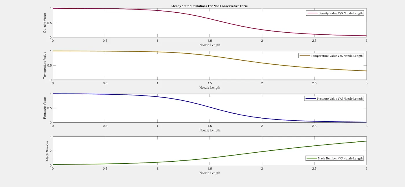
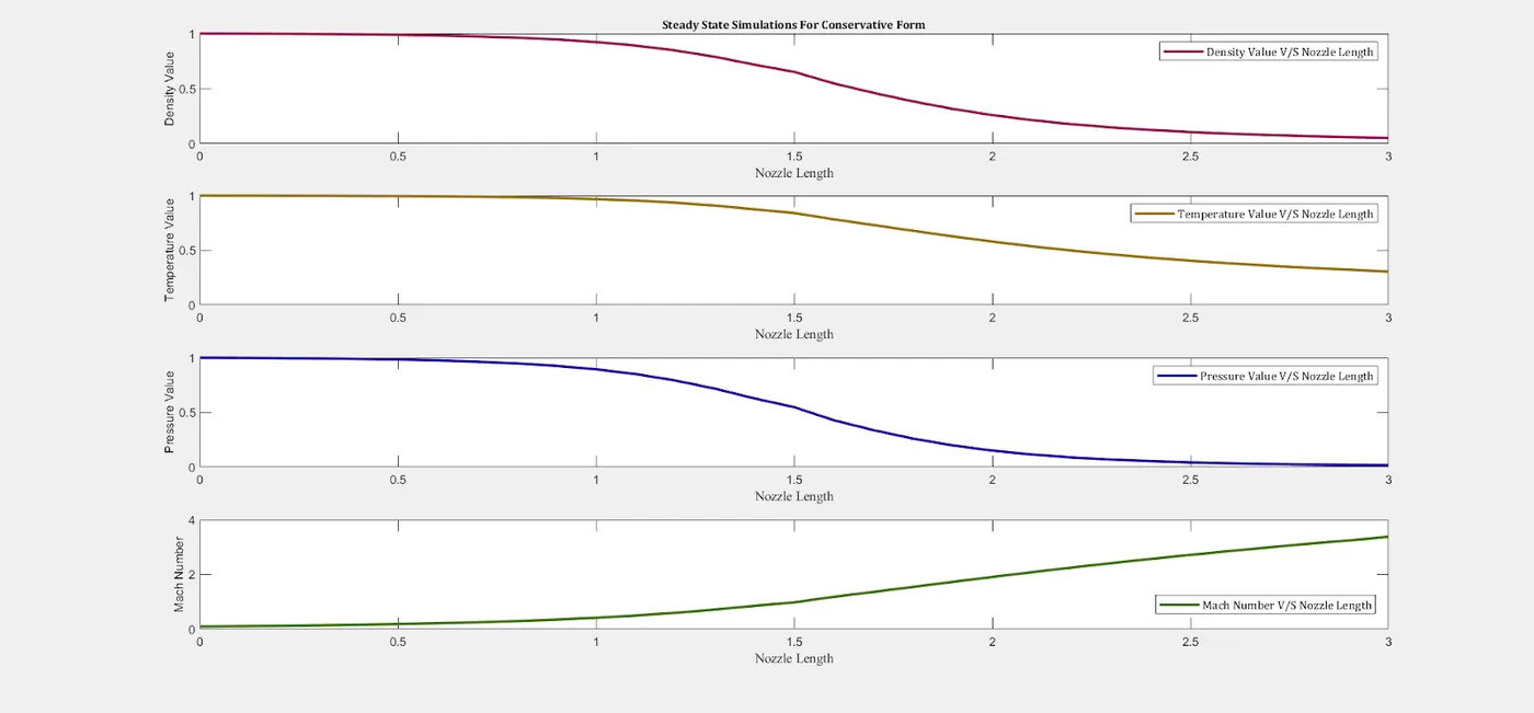
Steady-state distribution of primitive variables inside the Nozzle

Non Conservative Form

Conservative Form

Observation

⇒ Both the plots for conservative and non conservative are absolutely same, thus we can conclude that the flow distrbution through the nozzle length is same.

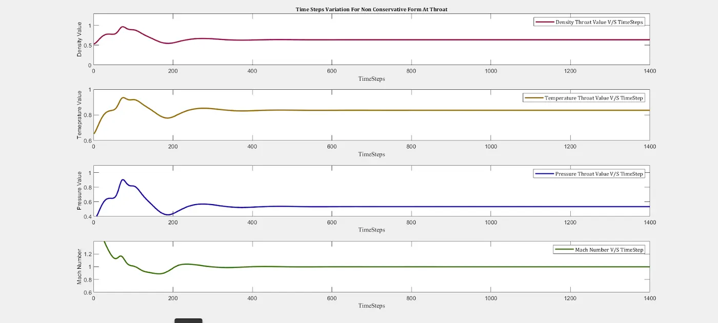
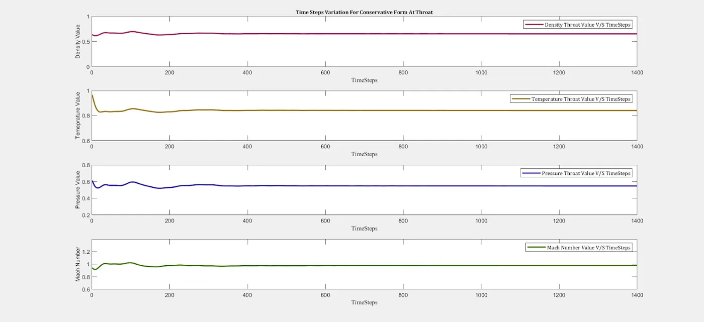
Time-Wise Variation of the Primitive Variables

Non Conservative Form

Conservative Form

Observation

⇒ From the above plots, we can observe that in case of non-conservative form, it requires a larger amount of time to achieve stable solution than conservative form.

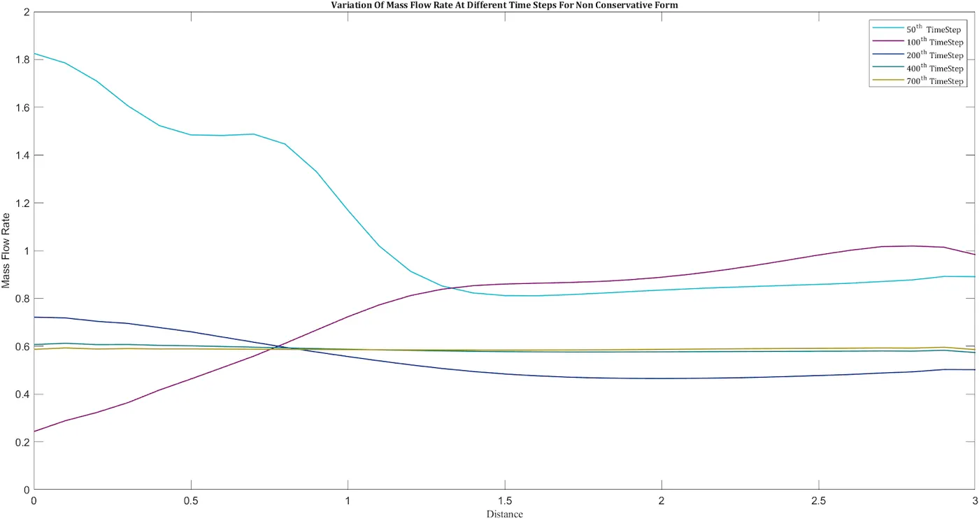
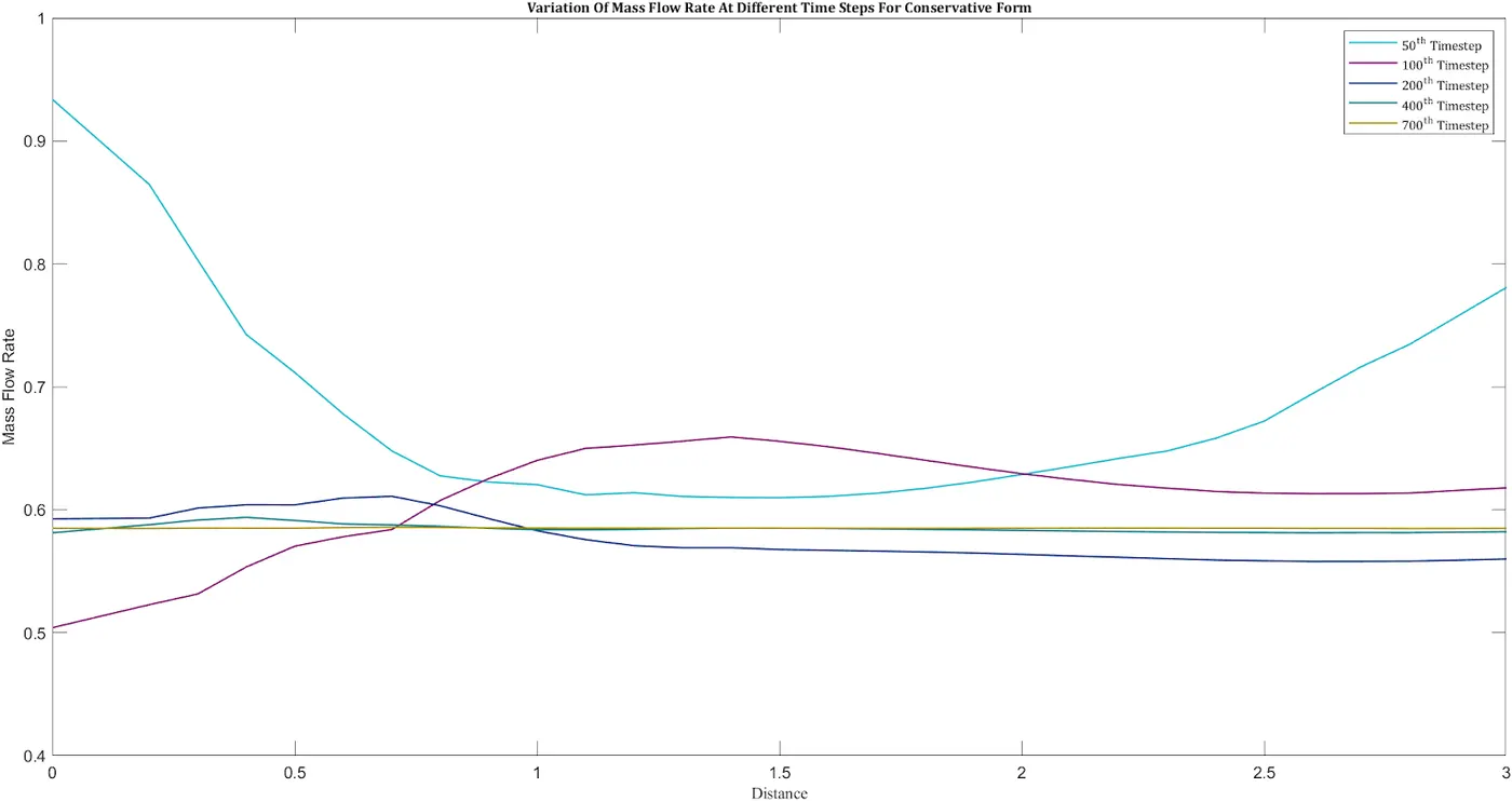
Variation of Mass flow Rate Distribution inside the nozzle at different time steps during the time-marching process

Non-Conservative Form

Conservative Form

Observation

⇒ From the above plots, we can observe that the Mass Flow Rate Converges After 400th Iterations For Both the cases.

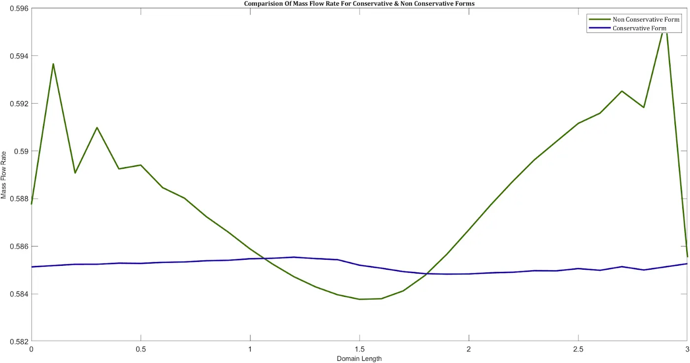
Comparison of Normalized Mass Flow Rate distributions of both forms

Observation

⇒ From the above plots, we can observe that the Non Conservative Method is oscillating at a very high pace throughout its nozzle nength, whereas In Conservative Method the plot is almost stable throughout its nozzle length.

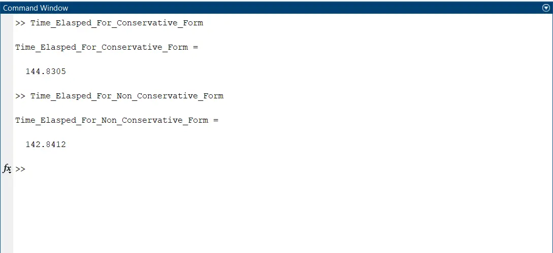
Time Taken By Conservative & Non-Conservative Form

GRID INDEPENDENCE TEST

Type	No Of Grid Points	Mass Flow Rate	Density	Pressure	Temperature	Velocity	Mach Number
Conservative	31	0.5852	0.6516	0.5478	0.8406	0.8981	0.9795
Non Conservative	31	0.5838	0.6387	0.5342	0.8365	0.9140	0.9994
Conservative	61	0.5829	0.6383	0.5331	0.8351	0.9132	0.9992
Non Conservative	61	0.5826	0.6376	0.5326	0.8354	0.9137	0.9997

From the above results, we can conclude the values are almost same, it is not varying much with the change in grid values.

Conclusion

We can observe that the conservative form is converging faster than the non-conservative form
We can also observe that the conservative form is producing a stable solution than non-conservative form.

Week 7 - Simulation of a 1D Supersonic nozzle flow simulation using Macormack Method

Ship work like this
in your own course.

Talk to a career counsellor

Ship work like thisin your own course.

Talk to a career counsellor

Ship work like this
in your own course.