Week 7 - Simulation of a 1D Supersonic nozzle flow simulation using Macormack Method

AIM:

• To simulate the isentropic flow through a quasi 1D subsonic-supersonic nozzle, and derive both the conservation and non-conservation forms of the governing equations ,solve them using the MacCormack's technique. Using Matlab.

OBJECTIVES:

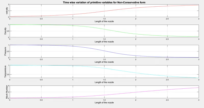
• Steady-state distribution of primitive variables inside the nozzle
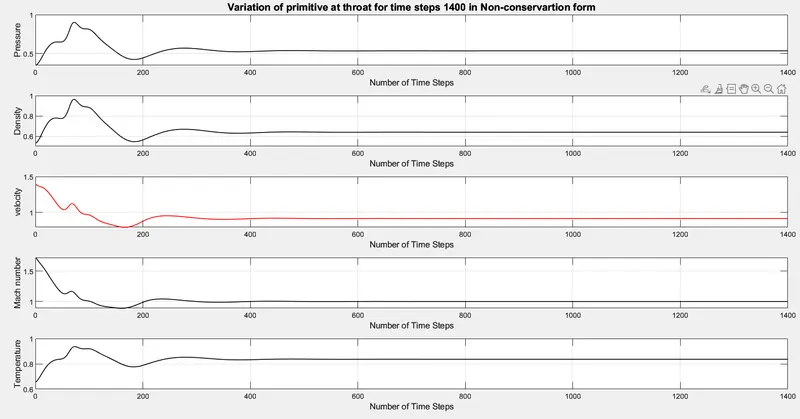
  Time-wise variation of the primitive variables
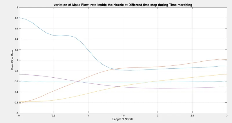
  3. Variation of Mass flow rate distribution inside the nozzle at different time steps during the time-marching process
  4. Comparison of Normalized mass flow rate distributions of both forms

PROCEDURE:

• QUASI ONE DIMENSIONAL NOZZLE FLOW:

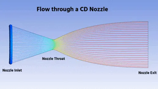
Quasi one dimensional implies that we still have variations of flow quantities in one direction only but we allow the cross section area of stream tubes to vary along the same direction as well. This means that we will be able to analyze axisymmetric channels with varying cross section areas such as for example convergent-divergent nozzles. One thing that is important to note is that for the equations to be valid the variation in cross section area has to be smooth.

GIF OF AN COVERGENT-DIVERGENT NOZZLE.

SUBSONIC AND SUPERSONIC FLOW:

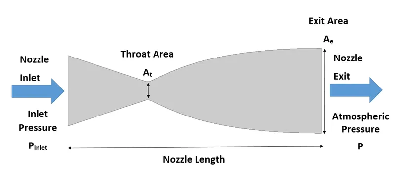
• Subsonic- Supersonic is known as convergent divergent nozzle. Supersonic and subsonic flow refer to the speed faster or slower than the speed of the sound. Anything going faster than the speed of the sound 343.2m/s, is supersonic flow. Anything going slower than the speed of the sound is called as the subsonic
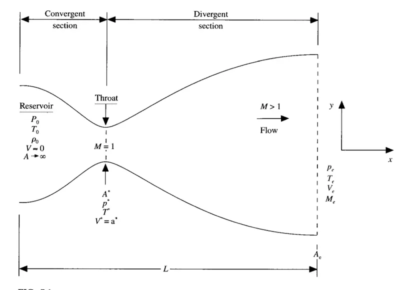
• The flow at the inlet to the nozzle comes from a reservoir where the pressure and temperature are denoted by `p_o and T_o`.The cross- sectional area of the reservoir is large (theoretically, A tends to inifinty ), and hence the velocity is very small (v tends to 0).Thus p0 and T0 are the stagnation values, or total pressure and total temperature, respectively. The flow expands isentropically to supersonic speeds at the nozzle exit, where the exit pressure, temperature, velocity, and Mach numver are denoted by pe, Te, Ve, and Me, respectively. The flow is locally subsonic in the convergence section of the nozzle, sonic at the throat (minimum area), and supersonic at the divergent section. The sonic flow (m=1) at the throat means that the local velocity is equal to the local speed of sound. We have at the throat V=V*=a*. Similarly, the sonic flow values of pressure and temperature are ddenoted by p* and T*, respectively. The area of the sonic throat is denoted by the A*. We assume the cross -sectional area is A, and the flow properties are uniform that section. Hence although the area of the nozzle changes as a function of distance along the nozzle, x, and therefore in reality the flow field is two-dimensional (the flow varies in the two-dimensional xy space), we make the assumption uniform flow properties across any given cross section. Such flow is defined as the quasi-one-dimensional flow.
• Before deriving into the governing equations, let us know the Conservation and Non-Conservation form therotically.

CONSERVATION AND NON-CONSERVATION.

• Both conservative and Non-conservative have three equation (that is ) Navier Stroke Equation.
• CONSERVATION OF MASS.
• MOMENTUM.
• ENERGY.
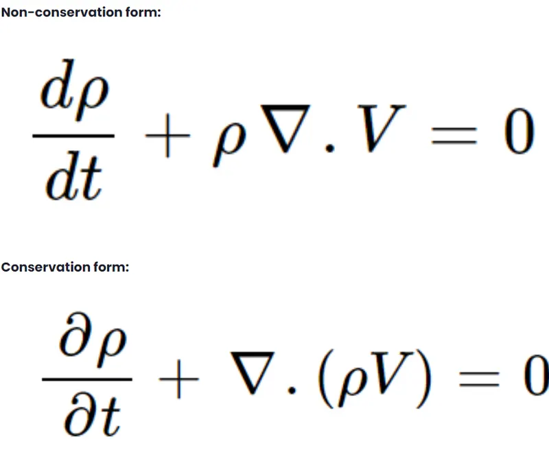
• For ex-ample let us consider the continuity equation derived for an infinitesimal control volume as shown as below.

DIFFERENCE BETWEEN THE BOTH FORMS.

FIRST DIFFERENCE.

• Time derivative term.
• Local derivative in conservative form is replaced by with the substantial derivative in non-conservation.
• In Conservative form, the control volume is fixed.
• So, the variation of density with the time is given t=by the local derivative.
• In Non-Conservative form, the control volume is moved.
• So, the time rate of change of density will be sum of the local derivative (variation due to unsteady native) and convective derivative (variation due to the moving control volume).

SECOND DERIVATIVE.

• Position of the nabla operator. It is called as the divergence or differential whose (Volume intensity of outward flux) of that the vector field.
• In Non-Conservative form the divergence operator is applied to the velocity and not the density.
• In convective, divergence operator is applied on both and there is no variable outside the divergence operator.
• In the continuity equation in the conservation form is that quantity that divergence operator is acting on (that is) is nothing but the mass flu(the rate of mass flow per unit area or the momentum per unit volume) which makes sense only the control volume is not moving. This applies for both the momentum and energy equation where the divergence operator acts on momentum flux and energy flux.

APPROACH METHOD.

• There are two methods deriving the governing equation in fluid dynamics.
• EULERIAN METHOD.
• LAGRANGIAN METHOD.

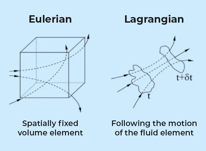
EULERIAN METHOD.

• Fixed point on the space and properties of fluid elements passing through it. (Conservation form).

LAGRANGIAN METHOD.

• We follow fluid particles as they travel through the flow. (Non-Conservative form).

COMPARING BOTH FORMS.

• PROGRAMMING
• ACCURACY.
• CONVERGENCE RATE.
• STABILITY.

PROGRAMMING CONVENIENCE.

• In programming point of view Non - Conservative form is better compared to the conservative form, because easy to program the equations are solved in the form of primitive variables (Density, Volume, Temperature) and their values can be applied directly.
• Whereas, In Conservative form the equation expressed in the flux variables and need to modify into the solution vector. Equation solved for solution vector and then the primitive variables are determined from them. This adds amount of complexity in conservation form.

ACCURACY.

• When looking at the primitive variables (Non_Conservative form is better and more accurate because primitive variables are solved directly from the governing equation).
• In Conservative form the primitive variables are computed only indirectly from the flux variables since the flux variables are solved directly solved for the conservation form.
• Increased number of calculations will lead more error due to computers constantly round off decimal values to machine precision.
• If we consider only the flux variables (Conservative form is better).

CONVERGENCE RATE.

• Primitive variables convergence to numerical steady state faster when using the non_Conservative form. That the dependent variables are in the non_conservative form might cause for that.
• Simulation time for Non_conseravtive form is shorter compared to the conservative form.

STABILITY.

• Stability plays an important role in the both forms.
• The equation we solve in CFD may not always be continuous. (There might exist discontinuous in some region of domain due to physical or mathematical nature of the equation we solving.
• The primitive variables like Density Temperature Volume experience sudden jump across these discontinuities.
• When the governing equation is expressed using the primitive variables (like in Nonconservative form), there may develop large gradient in the solution might cause the solution blow up.
• On the other hand, the flux variables possess the interesting property that remain constant across shocks or discontinuities.

MACCORMACK METHOD.

• Maccormack method is known as second order explicit Finite Difference Method which is widely used for discretization scheme for numerical solution of hyperbolic partial differential equations.
• It’s a two-step method. Easy to understand and program.

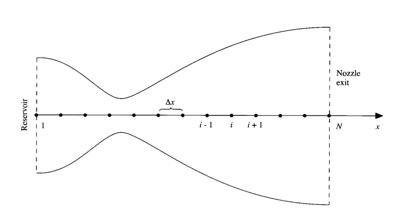
PREDICTOR STEP.

• In this step a provisional value is estimated and discretized for time derivative by Forward Difference of spatial derivative at time t + dt.

`f'(x) =( f(x+1) -f(x))/(dx)`

CORRECTOR STEP.

• In the corrector step, we again calculate the time derivative at t+ dt, this time substituting the obtained predicted value in the spatial derivative with backward difference.

`f'(x) = (f(x)-f(x-1))/(dx)`

• We can also use backward for predictor and forward difference scheme for corrector method.
• After this final value is calculated by the taking the average of the time derivatives obtained the predictor and corrector values.

GOVERING EQUATION.

• The governing equation for the Quasi One-Dimensional, Steady, Inviscid, Isentropic follow is given below.

CONTINUNITY EQUATION.

`rho_1*V_1*A_1 = rho_2*V_2*A_2`

MOMENTUM EQUATION.

`rho_1*A_1+rho_1*V_1^2*A_1 +int_(A1)^(A2) p*dA = p_2*A_2+rho_2*V_2^(2)*A_2`

ENERGY EQUATION.

`h_1+V_1^2/(2) = h_2+V_2^2/(2)`

where,

V - Velocity vector.

rho - Density of fluid.

A - Cross-sectional area.

p - Pressure for an ideal gas

`p = rho*R*T`

R - Gas constant.

T - Temperature.

h - Enthalpy for an ideal gas

`h = Cp*T`

Cp - specific heat constant.

• Since we are dealing with the one- dimensional inviscid flow for our nozzle problem. Assume that the flow properties are uniform across any given cross-sectional of the nozzle, in the reality the nozzle flow is two-dimensional flow with the change in cross sectional area with respect to function x, there will be the flow field variation in both the x and y directions. Therefore by assuming the twisted real [physics], the physical principle are justified with the assumption of qausi-1D flow. Integral form of governing equations to a constant volume which will be consistent with the quasi one-dimensional flow.

INTEGRAL FORM AND SURFACE AREA OF GOVERNING EQUATION.

CONTINUITY EQUATION.

`del/(delt) int int int_V rho*dV + del/(delt) int int rho*V*dS = 0`

MOMENTUM EQUATION.

`del/(delt) int int int_V(rho*u)*dV +del/(delt) (rho*u*V)*dS = -int int_sp*dS`

ENERGY EQUATION.

`del/(delt) int intint_Vrho*(e+(V^2/2))*dV+del/(delt)_S rho*(e+(V^2/2))*V*dS = -int int_S(p*V)*dS`

Since it is considered as the inviscid flow therefore the viscous terms are neglected.It is one dimensional flow.

u is the fluid velocity component at x direction, terms of velocity for the other directions are neglected.

e is the internal energy, for a ideal gas e = Cv*T where Cv is the specific heat at constant volume.

p is the pressure and rho is the density, for ideal gas p = rho*R*T where,R is the Gas constant.

V is the velocity vector, and is the control volume.

dS is the area vector, it is always Normal to the cross sectional area or any surface area.

GOVERNING EQUATION FOR QUASI 1 DIMENSIONAL INVISID, UNSTEADY, ISENTROPIC SUBSONIC-SUPERSONIC NOZZLE FLOW.

• In Non_Conservation form the control volume is moving along the fluid.

Continuity Equation.

`(del(rhoA))/(delt) + rhoA (delV)/(delx) + rhoV(delA)/(delx) +VA(delrho)/(delx) = 0`

Momentum Equation.

`rho(delV)/(delt) +rhoV(delV)/(delt) = -R(rho(delT)/(delx) +T(delrho)/(delx))`

Energy Equation.

`rhoC_v(delT)/(delt) +rhoVC_v(delT)/(delx) = -rhoRT(delV)/(delx) +V(del(lnA)/(delx))`

• In conversation form (control Volume is fixed)

Continuity Equation.

`del(rhoA)/(delt) +del(rhoAV)/(delx) = 0`

Momentum equation.

`del(rhoAV)/(delt) +(del(rhoAV^2))/(delx) = -A(delrho)/(delx)`

Energy equation.

`(del(rho*A*(e+(V^2/2))))/(delt) +(del(rho*A*V*(e+(V^2/2)) +pAV ))/(delx) = 0`

NON DIMENSIONAL PDE GOVERNING EQUATION.

• In fluid dynamics, Non-Dimensionalization of the equations is the conservation of the equations to a nondimensional form.This technique can ease the analysis of the problem at hand, and the reduce the number of free parameters. Small or large size of certain dimensionaless parameters indicates the importance of certain terms in the equations for the studied flow. This may provide possibilities to neglect terms in certain (areas of the considered flow).
• For the Nozzle Flows, the flow field variables are frequently expressed in terms of non-dimensional variables, such that Flow variables are referenced to their reservoir/inlet values.
• Non-Dimesional Variable for the governing equation with respect to the Flow-Feild Variables are as follows,

`T' = T/T_0 ; rho' = rho/rho_0 ; V' = V/a_0 ; A' = A/(A^star) ; x' =x/L ; t' =t/(L/a_0);`

where ,

`a_0 = (sqrtgamma*R*T)` speed of sound at the reservoir.

T' - Non dimensional Temperature,

T - Temperature of the fluid,

To - Temperature at the reservior.

rho' - Non dimensional density.

rho - Density of the fluid,

rho_o = Density at the reservior.

V' - Non dimensional velocity,

V - Velocity of the fluid,

A' - Non dimensional area,

A - Cross sectional area of the nozzle,

A* - Cross sectional area of nozzle throat.

x'- Non dimensional location,

x - location in the nozzle ,

L - length of the nozzle.

t'- Non Dimensional Time,

t - time.

NON DIMENSIONAL GOVERNING EQUATIONS.

NON-CONSERVATIVE FORM.

continuity equation.

`(delrho')/(delt') = -rho'(delV')/(delx')-rho'V'(del(lnA'))/(delx') -V'(delrho')/(delx')`

momentum equation.

`(delV')/(delt') = -V'(delV')/(delx') -(1/(gamma)*((delT')/(delx') +(T')/(rho')*(delrho')/(delx')))`

Energy Equation.

`(delT')/(delt') = - V'(delT')/(delx') -(gamma-1) *T'((delV')/(delx') +V' (del(lnA'))/(delx'))`

CONSERVATIVE FORM.

continuity equation

`(del(rho'A'))/(delt') +( del(rho' A'V'))/(delx') = 0`

Momentum Equation.

`(del(rho'A'V'))/(delt') + (del(rho'A'V'^2 +(1/gamma) rho'A'))/(delx') = 1/gamma *p' (delA')/(delx')`

Energy Equation.

`(del(rho'*A'*(e')/(gamma-1) + gamma/2 V'^2 ))/(delt') +(del(rho'*A'*V'*(e')/(gamma-1) + gamma/2 V'^2 +p'A'V'))/(delx')= 0/(delt')`

GENERIC FORM.

Continuity Equation.

`(delU_1)/(delt') = - (delF_1)/(delx')`

Momentum Equation

`(delU_2)/(delt') = - (delF_2)/(delx') +J_2`

Energy Equation.

`(delU_3)/(delt') = -(delF_3)/(delx')`

whereas ,

`U_1 = rho'*A';U_2 = rho' * A'*V' ; U_3 = rho'*A'*(((e')/(gamma-1)) +(gamma/2)*V'^2)`

`F_1 = rho' A'V'; F_2 = rho'A'V'^2+(1/gamma) rho'A' ; F_3 = rho'*A'*V'*((e)/(gamma-1) +(gamma)/2 V'^2) +rho'A'V'`

`rho' = U_1/(A') ; V' = U_2/(U_1) `

`T' = e' = (gamma-1)((U_3/(U_1) -gamma/(2) V'^2) ; p' = rho'T'`

BOUNDARY CONDITIONS.

• In order to exmaine the boundary conditions, we consider two infinitely weak mach waves at the boundary points, both proporgating with speed of sound a . One proporgating towards the left direction and other moving towards the right direction, both named as Left Running characteristic and right running characteristic.

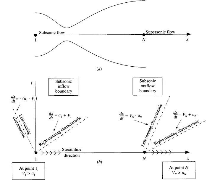
Subsonic Inflow Boundary Condition -

From the above figure we can see that at the Subsonic Inlet boundary, left running characteristic would be going towards left and the flow coming through inlet which is moving towards right, and will have the subsonic speed. The relative velocity of the left characteristic will be `-(a_1- V_1)` and relative velocity for the right running characteristic will be `(a_1+V_1)`. Hence, we can see here that the left running characteristic running characteristic is proporgating out of the nozzle region i.e. outside the domain of influence and right running characteristic proporgates inside the domain.

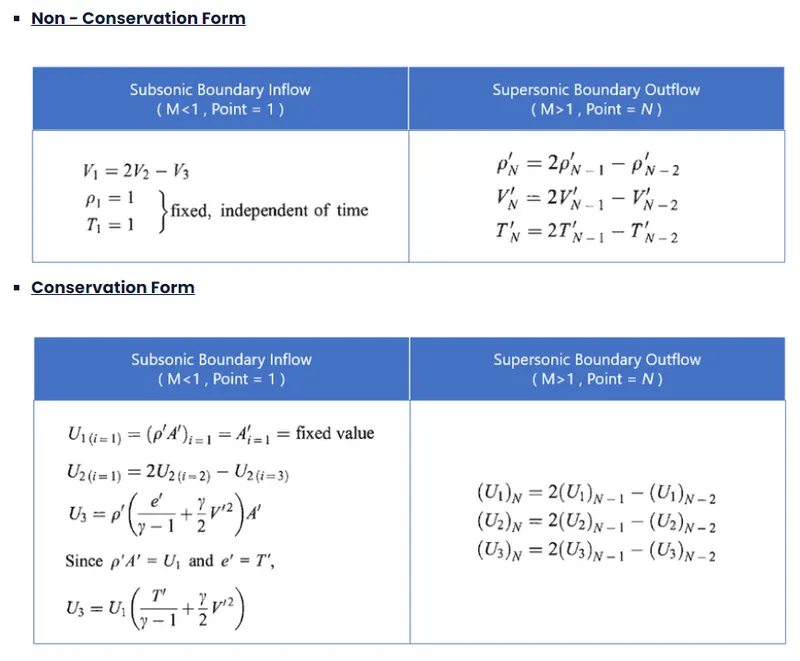
Therefore, as a conclusion, at the subsonic inlow boundary, we most stipulate the value of Two Fixed Flow-Field Variables that are independent of time, wheres the value of One other variable must be alowed to Float.

So, for the subsonic inlow boundary, we choose that the Density and the Energy Terms to be stipulated. And the Velocity term to be allowed to float with respect to time. The Velocity at the inlet boundary can be estimated by Linear Extrapolation, from the velocities obtained at inner nodes at every time step.

Supersonic Outflow Boundary Condition -

Now, by applying the same concept at the outflow boundary. The fluid flow is flowing towards right direction same as above, however now the speed of the stream is supersonic. So, the relative velocity of left characteristic `(V_N -a_N)` and right characteristic (`(V_N +a_N)` , both dominated dominated by the speed of the fluid flow. Hence, both of the characteristics are proporgating towards right diretion, and i.e. out of the Domain.

Therefore, at the Supersonic Outflow Boundary, since both the characteristic and the stream is going of the domain, So there are no Flow-Field Variables which require their values to be stipulates at the outflow boundary, Hence all variables must be allowed to Float at this boundary.

Here, at the outflow boundary all variables must be allowed to float, therefore we will calculate the variables using the Linear Extrapolation at every time Step.

TIME STEP CALCULATION.

The governing equations are hyperbolic and will be suing the explicit methods to solve it, and hence computing the time step is very critical as explicit time-integration method is sensitive to the timesteps. Having a wrong time steps will blow up solution and solution goes unstable. For stability purpose will be using courant number to calculate the time step to get a stable solution.

This is known as adaptive time step. In order to the avoid the solution to blow-up the time step should be calculated at every time step loop from the courant number.

Courant number C = 0.5

`dt = min (C*(dx/(a+v)))`

In Non-Dimensional form,

velocity of a sound `a' = a/a_0 ; Non Dimensional velocity v' = v/a_0`

where,

a = local velocity of sound.

a0 = velocity of sound.

a' = non-dimensional velocity of sound.

v' = non-dimensional velocity of fluid.

v = velocity of the fluid.

Now,

`a' = a/a_0 = sqrtT' = (T')^0.5`

`dt = min(C*(dx/(T'^0.5 +v')))`

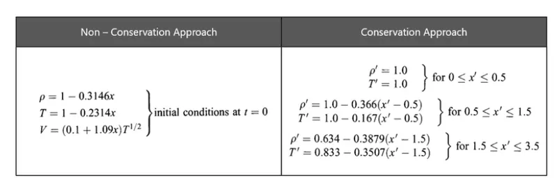
BOUNDARY CONDITIONS , INITIAL CONDITONS.

MAIN PROGRAM.

clear all
close all
clc
 
% Inputs 
% number of grids
 n = 31;
% length
 L = 3;
 x = linspace(0,L,n);
 dx = x(2)-x(1);
% To find the analytical solution
 analytical_solution = 0.579*ones(1,n);

% comparing conversative and non conservative form

[x, M_nc, rho_nc, v_nc, p_nc, T_nc, mfr_nc, rho_throat_nc,v_throat_nc, p_throat_nc, T_throat_nc, M_throat_nc, mfr_throat_nc] = non_conser();
[x, M_c, rho_c, v_c, p_c, T_c, mfr_c, rho_throat_c,v_throat_c, p_throat_c, T_throat_c, M_throat_c, mfr_throat_c] = conservative();


% Plotting non -conseravtive  form 

  figure(3)
  subplot (5,1,1)
  plot(x,v_nc,'color','r','linewidth',0.5)
  xlabel('Length of the nozzle','FontSize',10)
  ylabel('velcoity','FontSize',10)
  title ('Time wise variation of primitive variables for Non-Conservative form','FontSize',12)
  grid on
 
  subplot(5,1,2)
  plot(x,rho_nc,'color','g','linewidth',0.5)
  xlabel('Length of the nozzle','FontSize',10)
  ylabel('Density','FontSize',10)
  grid on

  subplot(5,1,3)
  plot(x,p_nc,'color','b','linewidth',0.5)
  xlabel('Length of the nozzle','FontSize',10)
  ylabel('Pressure','FontSize',10)
  grid on

  subplot(5,1,4)
  plot(x,T_nc,'color','c','linewidth',0.5)
  xlabel('Length of the nozzle','FontSize',10)
  ylabel('Temperature','FontSize',10)
  grid on
 
  subplot(5,1,5)
  plot(x,M_nc,'color','m','lineWidth',0.5)
  xlabel('Length of the nozzle','FontSize',10)
  ylabel('Mach Number','FontSize',10)
  grid on

  figure(4)

  subplot(5,1,1)
  plot(1:1400,p_throat_nc,'color','k','linewidth',1)
  xlabel('Number of Time Steps','FontSize',10)
  ylabel('Pressure','FontSize',10)
  title('Variation of primitive at throat for time steps 1400 in Non-conservartion form','FontSize',12)
  grid on

  subplot(5,1,2)
  plot(1:1400,rho_throat_nc,'color','k','linewidth',1)
  xlabel('Number of Time Steps','FontSize',10)
  ylabel('Density','FontSize',10)
  grid on

  subplot(5,1,3)
  plot(1:1400,v_throat_nc,'color','r','linewidth',1)
  xlabel('Number of Time Steps','FontSize',10)
  ylabel('velocity','FontSize',10)
  grid on
  
  subplot(5,1,4)
  plot(1:1400,M_throat_nc,'color','k','linewidth',1)
  xlabel('Number of Time Steps','FontSize',10)
  ylabel('Mach number','FontSize',10)
  grid on

  subplot(5,1,5)
  plot(1:1400,T_throat_nc,'color','k','linewidth',1)
  xlabel('Number of Time Steps','FontSize',10)
  ylabel('Temperature','FontSize',10)
  grid on

% Plotting conseravtive form 

  figure(5)
  subplot (5,1,1)
  plot(x,v_c,'color','r','linewidth',1.5)
  xlabel('Length of the nozzle')
  ylabel('velcoity')
  title ('Time wise variation of primitive variables for Conservative form','FontSize',12)
  grid on 
 
  subplot(5,1,2)
  plot(x,rho_c,'color','r','linewidth',1.5)
  xlabel('Length of the nozzle')
  ylabel('Density')
  grid on 

  subplot(5,1,3)
  plot(x,p_c,'color','b','linewidth',1.5)
  xlabel('Length of the nozzle')
  ylabel('Pressure')
  grid on

  subplot(5,1,4)
  plot(x,T_c,'color','g','linewidth',1.5)
  xlabel('Length of the nozzle')
  ylabel('Temperature')
  grid on 
 
  subplot(5,1,5)
  plot(x,M_c,'color','g','linewidth',1.5)
  xlabel('Length of the nozzle')
  ylabel('Mach Number')
  grid on

  figure(6)

  subplot(5,1,1)
  plot(1:1400,p_throat_c)
  xlabel('number of time steps')
  ylabel('pressure')
  grid on

  subplot(5,1,2)
  plot(1:1400,rho_throat_c)
  xlabel('number of time steps')
  ylabel('density')
  grid on 


  subplot(5,1,3)
  plot(1:1400,v_throat_c)
  xlabel('number of time steps')
  ylabel('velocity')
  grid on 

  
  subplot(5,1,4)
  plot(1:1400,M_throat_c)
  xlabel('number of time steps')
  ylabel('mach number')
  grid on


  subplot(5,1,5)
  plot(1:1400,T_throat_c)
  xlabel('numbe of time steps')
  ylabel('temperature')
  grid on 

  figure (7)
  plot(x,mfr_c,'color','k')
  hold on   
  plot(x,mfr_nc,'color','r')
  hold on 
  plot(x,analytical_solution,'color','g')
  xlabel('length of the nozzle')
  ylabel('mass flow rate')
  grid on

NON -CONSERVATION FORM.

function [x, M, rho, v, p, T, mfr, rho_throat,v_throat, p_throat, T_throat, M_throat, mfr_throat] = non_conser()
 

% Inputs 
% length of the domain 
L = 3;
% number of grid points
n = 31;
x = linspace(0,L,n);
dx = x(2)-x(1);
% Ratio of specfic heats (Cp/Cv) for air standard conditions
gamma = 1.4;

% calculate the initial profile
% density 
rho = 1-0.3146*x;
% temperature 
T  = 1-0.2314*x;
% velocity 
v = (0.1+1.09*x).*T.^0.5;
% nozzle shape 
a = 1+2.2*(x-1.5).^2;
% Pressure 
p = rho.*T;
% mass flow rate  
mfr = rho.*v.*a;
% mach number 
M = v./(T.^0.5);
% courrant number 
C = 0.5;
% Throat values 
throat = find (a==1);

% Time step
% number of time steps 
 nt = 1400;
% To calculate the time step 
% dt = min(C*dx)./(a+v);
% alternate form 
dt = min((C*dx)./((sqrt(T)+v)));


% Outer time loop 
for k = 1:nt

    rho_old = rho;
    v_old   = v;
    T_old   = T;
    M_old = M;
    p_old = p;
    
    % Predictor method 
    for j = 2:n-1

        dvdx    = (v(j+1)-v(j))/(dx);
        drhodx  = (rho(j+1)-rho(j))/(dx);
        dTdx    = (T(j+1)-T(j))/(dx);
        dlogadx = (log(a(j+1))-log(a(j)))/(dx);
        
        % continuity equation 
        drhodt_p(j) = -rho(j)*dvdx-rho(j)*v(j)*dlogadx-v(j)*drhodx;

        % momentum equation 
        dvdt_p(j)  = -v(j)*dvdx-(1/gamma)*(dTdx+(T(j)/rho(j))*drhodx);

        % energy equation 
        dTdt_p(j)  = -v(j)*dTdx-((gamma-1)*T(j))*(dvdx+v(j)*dlogadx);

        % solution update 
        rho(j) = rho(j)+drhodt_p(j)*dt;
        v(j)   = v(j)+dvdt_p(j)*dt;
        T(j)   = T(j)+dTdt_p(j)*dt;

    end

    % corrector step 
     for j = 2:n-1

        dvdx    = (v(j)-v(j-1))/(dx);
        drhodx  = (rho(j)-rho(j-1))/(dx);
        dTdx    = (T(j)-T(j-1))/(dx);
        dlogadx = (log(a(j))-log(a(j-1)))/(dx);
        
        % continuity equation 
        drhodt_c(j) = -rho(j)*dvdx-rho(j)*v(j)*dlogadx-v(j)*drhodx;

        % momentum equation 
        dvdt_c(j)  = -v(j)*dvdx-(1/gamma)*(dTdx+(T(j)/rho(j))*drhodx);

        % energy equation 
        dTdt_c(j)  = -v(j)*dTdx-((gamma-1)*T(j))*(dvdx+v(j)*dlogadx);

     end

     % calculate  the average time derivative 
     drhodt = 0.5*(drhodt_p+drhodt_c);
     dvdt   = 0.5*(dvdt_p+dvdt_c);
   
     dTdt   = 0.5*(dTdt_p+dTdt_c);


     % calculate the final solution 

    for i = 2:n-1 
        rho(i) = rho_old(i)+drhodt(i)*dt;
        v(i)   = v_old(i)+dvdt(i)*dt;
        T(i)   = T_old(i)+dTdt(i)*dt;
    end
    
   
    % apply the boundary conditions 
    % for inlet 
    v(1) = 2*v(2)-v(3);
    % for oulet 
    rho(n) = 2*rho(n-1)-rho(n-2);
    v(n) = 2*v(n-1)-v(n-2);
    T(n) = 2*T(n-1)-T(n-2); 

    % calculate the pressure,mach number and mass flow rate

     % Pressure 
     p = rho.*T;
     % mass flow rate 
     mfr = rho.*v.*a;
     % mach number 
     M = v./(T.^0.5);

     % calculate the throat value 

      rho_throat(k)=rho(throat);
      v_throat(k) = v(throat);
      p_throat(k) = p(throat);
      T_throat(k) =T(throat);
      M_throat(k) = M(throat);
      mfr_throat(k)= mfr(throat);

     % For each time step definig the mass flow rate    
     figure(1)

     if k == 50
         plot(x,mfr)
         hold on 

     elseif k == 100
         plot(x,mfr)
         hold on 

     elseif k == 150
         plot(x,mfr)
         hold on

     elseif k == 200
         plot(x,mfr)
         hold on 

     elseif k == 700
         plot(x,mfr)
         hold on 

     elseif k == 1400
         plot(x,mfr)
         hold on 
         xlabel('Length of Nozzle','FontSize',12,'linewidth',1.5)
         ylabel('Mass Flow Rate','FontSize',12,'linewidth',1.5)
         title ('variation of Mass Flow  rate inside the Nozzle at Different time step during Time marching','FontSize',14)
         grid on
     end
         
end

end

CONSERVATIVE FORM .

function [x, M, rho, v, p, T, mfr, rho_throat,v_throat, p_throat, T_throat, M_throat, mfr_throat] = conservative()

% Inputs 
% length of the domain 
L = 3;
% number of grid points
n = 31;
x = linspace(0,L,n);
dx = x(2)-x(1);
% Ratio of specfic heats (Cp/Cv) for air standard conditions
gamma = 1.4;



% Initial conditions 
%  rho = 1; 
%  T = 1;
% 
%  rho = 1-0.366*(x-0.5);  
%  T = 1-0.167*(x-0.5);
% 
%  rho = 0.634-0.3879*(x-1.5); 
%  T = 0.833 - 0.3507*(x-1.5);


for i = 1:length(x)
  if x(i)>=0 && x(i)<=0.5
    rho(i) = 1;
    T(i) = 1;

  elseif x(i)>=0.5 && x(i)<=1.5
    rho(i)    = 1-0.366*(x(i)-0.5);
    T(i)      = 1-0.167*(x(i)-0.5);
    
  elseif x(i)>=1.5 && x(i)<=3.5
    rho(i)    = 0.634-0.3879*(x(i)-1.5);
    T(i)      = 0.833-0.3507*(x(i)-1.5);
  end
end

% Initial profile 
% nozzle shape 
a = 1+2.2*(x-1.5).^2;
% velocity 
v = 0.59./(rho.*a);
% Pressure 
p = rho.*T;
% mass flow rate  
mfr = rho.*v.*a;
% mach number 
M = v./(T.^0.5);
% courrant number 
C = 0.5;

% To find the throat
throat =find(a==1);

    
% calculate the initial profile 
U1 = rho.*a;
U2 = rho.*a.*v;
U3 = rho.*(T/(gamma-1)+(gamma/(2)).*v.^2).*a;

% time steps 
nt = 1400;
dt = min((C*dx)./((sqrt(T)+v)));

% outer time loop 
for k = 1:nt 
    U1_old = U1;
    U2_old = U2;
    U3_old = U3;

    rho_old = rho;
    v_old   = v;
    T_old   = T;
  
    %  calculate Flux vectors 

    F1 = U2;
    F2 =((U2.^2)./(U1))+((gamma-1)/(gamma))*(U3-((gamma/2)*((U2.^2)./(U1))));
    F3 = ((gamma*U2.*U3)./(U1)) -((gamma*(gamma-1))/(2))*((U2.^3)./(U1.^2));

    % predictor step 
     for j = 2:n-1

      % source term
      J2_p(j) = (1/gamma)*(rho(j)).*(T(j)).*(a(j+1)-a(j))/(dx);      

      % continuity equation 
      dU1dt_p(j) = -(F1(j+1)-F1(j))/(dx);

      % momentum equation
      dU2dt_p(j) = -(F2(j+1)-F2(j))/(dx)+J2_p(j);

      % energy equation 
      dU3dt_p(j) = -(F3(j+1)-F3(j))/(dx);

      % Solution update 
      U1(j) = U1(j)+dU1dt_p(j)*dt;
      U2(j) = U2(j)+dU2dt_p(j)*dt; 
      U3(j) = U3(j)+dU3dt_p(j)*dt;

     end

    % Updating the primitive variables
    rho = U1./a;
    v = U2./U1;
    T  = (gamma-1)*(U3./(U1)-(gamma/(2))*v.^2);
    

    % Updating the flux vectors values 
    F1 = U2;
    F2 =((U2.^2)./(U1))+((gamma-1)/(gamma))*(U3-((gamma/2)*((U2.^2)./(U1))));
    F3 = ((gamma*U2.*U3)./(U1))-((gamma*(gamma-1))/(2))*((U2.^3)./(U1.^2));

    % Corrector step 
    for j = 2:n-1

      % source term
      J2_c(j) = (1/gamma)*(rho(j)).*(T(j)).*(a(j)-a(j-1))/(dx);      

      % continuity equation 
      dU1dt_c(j) = -(F1(j)-F1(j-1))/(dx);

      % momentum equation
      dU2dt_c(j) = -(F2(j)-F2(j-1))/(dx)+J2_c(j);

      % energy equation 
      dU3dt_c(j) = -(F3(j)-F3(j-1))/(dx);

    end
  
     % calculate the average time derivative 

     dU1dt = 0.5*(dU1dt_p+dU1dt_c);
     dU2dt = 0.5*(dU2dt_p+dU2dt_c);
     dU3dt = 0.5*(dU3dt_p+dU3dt_c);

     % final solution
     
     for i = 2:n-1
         U1(i) = U1_old(i)+dU1dt(i)*dt;
         U2(i) = U2_old(i)+dU2dt(i)*dt;
         U3(i) = U3_old(i)+dU3dt(i)*dt;
     end

     % Applying the boundary conditions 
     % Inlet 

     U1(1) = rho(1).*a(1);
     U2(1) = 2*U2(2)-U2(3);
     U3(1) = U1(1)*(T(1)./(gamma-1))+(gamma/(2))*(v(1).^2);

     % Outlet 
     U1(n) = 2*U1(n-1)-U1(n-2);
     U2(n) = 2*U2(n-1)-U2(n-2); 
     U3(n) = 2*U3(n-1)-U3(n-2);

     % calculate the primitive variables

     rho = U1./a;
     v   = U2./U1;
     T   = (gamma-1)*(U3./(U1)-(gamma/(2))*v.^2);

     % Pressure 
      p = rho.*T;
     % mass flow rate  
      mfr = rho.*v.*a;
     % mach number 
      M = v./(T.^0.5);

    % calculate the throat value
      rho_throat(k)=rho(throat);
      v_throat(k) = v(throat);
      p_throat(k) = p(throat);
      T_throat(k) =T(throat);
      M_throat(k) = M(throat);
      mfr_throat(k)= mfr(throat);

     % For each time step definig the mass flow rate    
      figure(2)
     
     if k == 50
         plot(x,mfr)
         hold on 

     elseif k == 100
         plot(x,mfr)
         hold on 

     elseif k == 150
         plot(x,mfr)
         hold on

     elseif k == 200
         plot(x,mfr)
         hold on 

     elseif k == 700
         plot(x,mfr)
         hold on 

     elseif k == 1400
         plot(x,mfr)
         hold on
         xlabel('Length of Nozzle','FontSize',12,'linewidth',1.5)
         ylabel('Mass Flow Rate','FontSize',12,'linewidth',1.5)
         title ('variation of Mass Flow  rate inside the Nozzle at Different time step during Time marching for conseravtion form ','FontSize',14)
         grid on 
     end
end
end

OUTPUTS.

NON CONSERVATIVE FORM.

CONSERVATIVE FORM.

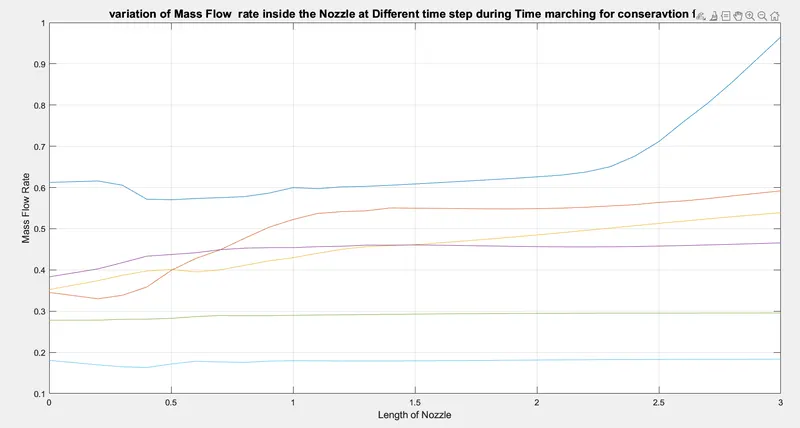
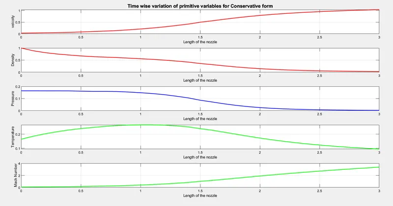
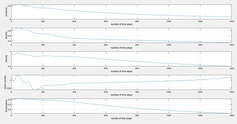
COMPARISON.

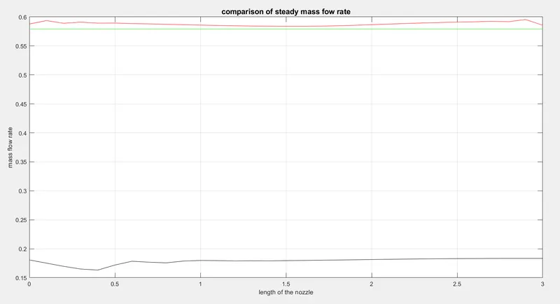
CONCLUSION.

• Hence the Non-conservation and conseravtion form of governing eqautions id derived and the solution is stable.
• The Non-conservative form has better convergence compare to the conservative form.
• The conservative form gives more accurate, smoother and stable,comparing to the conservative form
• In Non conserative form the direct approach is used,but in conservative form flux variables is introduce so it takes the more computational time.