Week 7 - Simulation of a 1D Super-sonic nozzle flow simulation using Macormack Method
Aim:To simulate isentropic flow through quasi 1-dimensional subsonic_supersonic nozzle.
Objective:
- Derive a equation for continuity, momentum, and energy for both conservative and non-conservative form.
- Write a matlab code for all the above derived equations. structure a matlab code according to MacCormack's technique.
- Plot for all the primitive variables and compare the results in between conservative and non-conservative forms.
- Define grid dependence and check for it.
- Calculate and plot mass flow rate at different time steps.
Introduction
What is isentropic process?
A process which is both adiabatic(No heat transfer takes place), and reversible(whose direction can be reversed to return the system to its original state).
Quasi 1-dimensional states that the simulation is partially one dimensional. which can be understood by taking nozzle into consideration, the nozzle flow is always an 2-dimensional flow but here we consider the parameters does not vary in y-direction.
subsonic-supersonic flow:
subsonic and supersonic refers to speed above a below the speed of sound which we will be considering in our nozzle flow. Inbetween subsonic and supersonic we do have transonic range which will also be included in our flow simulation.
We consider a steady state, isentropic flow through a convergent-divergent nozzle. The flow at inlet to the nozzle comes from the reservoir the pressure a temperature at reservoir is pi, and ti, respectively . The flow expands isentropically to supersonic speeds at nozzle outlet, where the exit velocity, pressure, mach number, and temperature are denoted at p0, t0 ,m0,and v0, respectively. The flow is subsonic in convergent portion sonic/transonic in throat and supersonic in divergent portion. the sonic at throat means the velocity at this section is equal to local speed of sound.
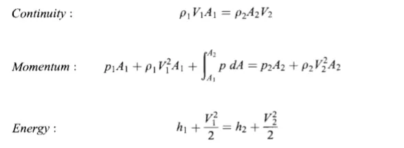
The governing continuity, momentum, and energy equations for quasi 1-dimensional, steady, isentropic flow are given as;
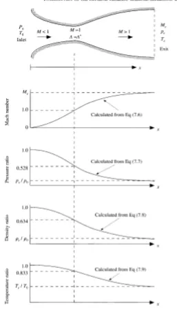
The plots expected for mach number, prressure, temperature, and density over the length of nozzle:
MacCormack's technique:
There are various simulation techniques in CFD among which macCormack's method is one of the simplest technique to apply for nozzle flow problem.
General structure of macCormack's method:
The macCormack's loop:
Step-1: The first step in macCormack's method is to calculate predictor step, to calculate predictor step we use governing equations and apply forward differencing to it.
Step-2: Updating the value of primitive variables used in governing equation.
Step-3: Using updated values for primitive variables in corrector step, the major difference is applying backward differencing to it.
Step-4: Calculating the average value of the time derivative for all the equation obtained by arithematic mean of predicitor and corrector values.
Step-5: Updating the values of primitive variables.
Step-6: Applying initial and boundary conditions.
Equations for conservative and non-conservative forms:
The final equations we get are in terms of dimensional variables, using dimensional variable is good choice but it makes equation look bit complicated, Hence the equation we will be using in our code are in terms of dimensionless quantities.
Governing equation for non-conservative form:



Governing equation for conservative form:
continuity equation:
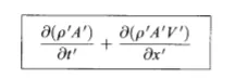
Momentum equation:

Energy equation:

The equations for quasi-one-dimensional flow can be expressed in generic form in terms of solution vector U, the flux vector F, the source term J as follows:
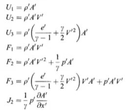
Using above generic equations in continuity, momentum and energy equation we get:
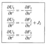
The solution we get are in form of solution vector U1,U2,and U3. we should decode this into primitive variables such as:
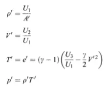
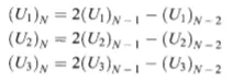
Final step is applying boundary and initial conditions:
Initial and boundary conditions for conservative form:
Initial conditions:
A = 1 + 2.2*(x - 1.5)^2
ρ = 1 - 0.3146*x
T = 1 - 0.2314*x
V = (0.1+1.09*x)*T^(0.5)
Boundary conditions:
Inflow:
V(1) = 2*V(2) - V(3)
Outflow:`rho`
V(n) = 2*V(n-1) - V(n-2)
T(n) = 2*T(n-1) - T(n-2)
ρ(n) = 2*ρ(n-1) - ρ(n-1)
Initial and boundary conditions for non-conservative form:
Initial condition:
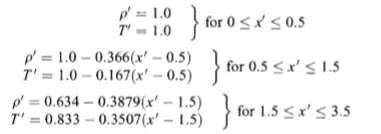
Boundary conditions:
Inflow:


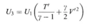
Outflow:
Steps/logic:
- Define input values such as length of nozzle, gamma, CFL number etc.
- Create a array of x through the length of nozzle.
- Define initial conditions.
- Calculate the value of time step.
- Create a time loop.
- Applying the macCormack's method.
- Plotting the results.
Main code for executing both conservative and non-conservative form:
close all
clear all
clc

%inputs
L=3; %length of the nozzle
n=31;
x=linspace(0,L,n);
dx=x(2)-x(1);

%area for 0=<x=<3

gamma = 1.4;
CFL = 0.5;  %courant fredrich lewyish number for stablility
nt = 1400;  %time steps

%Dimension of throat
Throat = (n-1)/2;
th = Throat;

%Iteration number

 iteration = input('enter the type of method =  ')


 if (iteration==1)
     [v_i,T_i,rho_i,M_i,mf_i,p_i,v_th_i,T_th_i,rho_th_i,M_th_i,mf_th_i,p_th_i] = conservative_solver(x,dx,nt,gamma,n,CFL,th)
 end
 if (iteration==2)
     [v_nc,T_nc,rho_nc,M_nc,m_nc,p_nc,v_th_nc,T_th_nc,rho_th_nc,M_th_nc,m_th_nc,p_th_nc] = nonconservative_solver(x,dx,nt,gamma,n,CFL,th)
 end
Matlab code for conservative form:
function [v_i,T_i,rho_i,M_i,mf_i,p_i,v_th_i,T_th_i,rho_th_i,M_th_i,mf_th_i,p_th_i] = conservative_solver(x,dx,nt,gamma,n,CFL,th)

%initial condition
for i= 1:length(x)
    if x(i)>=0 && x(i)<=0.5
        rho_i(i) = 1;
        T_i(i) = 1;
    else if x(i)>=0.5 && x(i)<=1.5
        rho_i(i) = 1 - 0.366*(x(i) - 0.5);
        T_i(i) = 1 - 0.167*(x(i) - 0.5);
    else if x(i)>=1.5 && x(i)<=3.5
        rho_i(i) = 0.634 - 0.3879*(x(i) - 1.5);
        T_i(i) = 0.833 - 0.3507*(x(i) - 1.5);
        end
      end
    end
end
A= 1+(2.2*(x-1.5).^2);


%values of primitive variables at t=0
%velocity
v_i = (0.59./(rho_i.*A));

%pressure
p_i = rho_i.*T_i;

%mach number
M_i = v_i./(T_i.^(0.5));

%mass flow rate
mf_i = rho_i.*v_i.*A;

%time step calculation
for i=1:n
    dt_cal(i) = CFL*(dx/((T_i(i).^(0.5))+(v_i(i))));
end
dt_i = min(dt_cal);

%Calculating solution vectors for initial condition
U1 = rho_i.*A;
U2 = rho_i.*A.*v_i;
U3 = rho_i.*(((T_i)/(gamma-1))+((gamma/2)*(v_i.^2))).*A;

nt=1400;
%time loop for carrying macormack method
for j= 1:nt

    %specifying the initial value because at every loop this value get updated
    U1_old =U1;
    U2_old =U2;
    U3_old =U3;

    %flux value in terms of u1,u1,and u3
    F1 = U2;
    F2 = ((U2.^2)./U1)+(((1/gamma)*(gamma-1)).*(U3-((gamma/2)*((U2.^2)./U1))));
    F3 = (((gamma*U2.*U3)./U1)- (((gamma*(gamma-1))/2)*((U2.^3)./(U1.^2)))) ;


    %predictor step
    for b= 2:n-1
        J2(b) = (1/gamma)*rho_i(b).*T_i(b).*((A(b+1)-A(b))/dx);
        du1_dt_p(b) = -((F1(b+1) - F1(b))/dx);
        du2_dt_p(b) = -((F2(b+1) - F2(b))/dx) + J2(b);
        du3_dt_p(b) = -((F3(b+1) - F3(b))/dx);

        U1(b) = U1(b)+((du1_dt_p(b))*dt_i);
        U2(b) = U2(b)+((du2_dt_p(b))*dt_i);
        U3(b) = U3(b)+((du3_dt_p(b))*dt_i);
    end

    rho_i = U1./A;
    v_i = U2./U1;
    T_i = (gamma-1)*((U3./U1) - ((gamma/2)*(v_i).^2));

    F1 = U2;
    F2 = ((U2.^2)./U1)+(((1/gamma)*(gamma-1)).*(U3-((gamma/2)*((U2.^2)./U1))));
    F3 = (((gamma*U2.*U3)./U1)- (((gamma*(gamma-1))/2)*((U2.^3)./(U1.^2)))) ;

%corrector method
for b= 2:n-1
        J2(b) = (1/gamma)*rho_i(b).*T_i(b).*((A(b)-A(b-1))/dx)
        du1_dt_c(b) = -((F1(b) - F1(b-1))/dx);
        du2_dt_c(b) = -((F2(b) - F2(b-1))/dx) + J2(b) ;
        du3_dt_c(b) = -((F3(b) - F3(b-1))/dx);
end
%calculating average time step
du1_dt_avg = 0.5*(du1_dt_p+du1_dt_c)
du2_dt_avg = 0.5*(du2_dt_p+du2_dt_c)
du3_dt_avg = 0.5*(du3_dt_p+du3_dt_c)

%Updating the value of solution vectors
 for i=2:n-1
    U1(i)= U1_old(i)+((du1_dt_avg(i))*(dt_i));
    U2(i)= U2_old(i)+((du2_dt_avg(i))*(dt_i));
    U3(i)= U3_old(i)+((du3_dt_avg(i))*(dt_i));
end

%boundary conditions
%inflow boundary  conditions
 U1(1) = rho_i(1)*A(1);
 U2(1) = 2*U2(2) - U2(3);
 v_i(1) = U2(1)./U1(1);
 U3(1) = U1(1)*((T_i(1)/(gamma-1))+((gamma/2)*v_i(1)^2));

 %outflow boundary condition
 U1(n) = 2*U1(n-1) - U1(n-2);
 U2(n) = 2*U2(n-1) - U2(n-2);
 U3(n) = 2*U3(n-1) - U3(n-2);

 %Updating primitive variables
 rho_i = U1./A;
 v_i = U2./U1;
 T_i = (gamma-1)*((U3./U1) - ((gamma/2)*v_i.^2));

 %Flow properties
 M_i = v_i./(T_i.^(0.5));
 p_i = rho_i.*T_i;
 mf_i = rho_i.*v_i.*A;

 %Values at throat
v_th_i(j) = v_i(th);
T_th_i(j) = T_i(th);
M_th_i(j) = M_i(th);
p_th_i(j) = p_i(th);
rho_th_i(j) = rho_i(th);
mf_th_i(j) = mf_i(th);

%plotting the mass flow rate at different time steps
figure(1)
hold on
if j==50
    plot(x,mf_i,'color','r')
elseif j==100
        plot(x,mf_i,'color','g')
elseif j==200
            plot(x,mf_i,'color','b')
elseif j==300
            plot(x,mf_i,'color','m')
elseif j==500
            plot(x,mf_i,'color','c')
            xlabel('array of x values')
            ylabel('mass flow rate for different time steps')
            legend('50nt','100nt','200nt','300nt','500nt')
end
end

%plotting the variation of primitive variables with length of nozzle
hold on
figure(2)
subplot(2,2,1)
plot(x,rho_i)
title('density vs length of nozzle')
xlabel('length of nozzle')
ylabel('density')

subplot(2,2,2)
plot(x,p_i)
title('pressure vs length of nozzle')
xlabel('length of nozzle')
ylabel('pressure')

subplot(2,2,3)
plot(x,T_i)
title('temperature vs length of nozzle')
xlabel('length of nozzle')
ylabel('temperature')

subplot(2,2,4)
plot(x,M_i)
title('Mach number vs length of nozzle')
xlabel('length of nozzle')
ylabel('Mach number')

%variation of primitive variable with time step near a throat
hold on
figure(3)
subplot(2,2,1)
plot(linspace(1,nt,nt),rho_th_i)
title('density at throat vs time step')
axis([0 1400 0.6 0.8])
xlabel('Time step')
ylabel('density at throat')

subplot(2,2,2)
plot(linspace(1,nt,nt),T_th_i)
title('Temperature at throat vs time step')
axis([0 1400 0.8 0.9])
xlabel('Time step')
ylabel('Temperature at throat')

subplot(2,2,3)
plot(linspace(1,nt,nt),p_th_i)
title('pressure at throat vs time step')
axis([0 1400 0.55 0.7])
xlabel('Time step')
ylabel('pressure at throat')

subplot(2,2,4)
plot(linspace(1,nt,nt),M_th_i)
title('Mach number at throat vs time step')
axis([0 1400 0.8 0.9])
xlabel('Time step')
ylabel('Mach number at throat')


end
PLOTS:
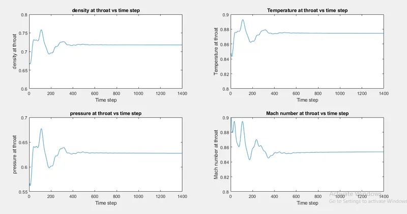
Plot of primitive variables vs time step:
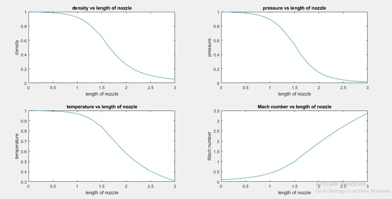
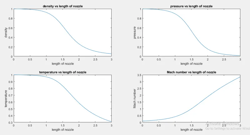
Plot for variation of primitive variables with the length of nozzle:
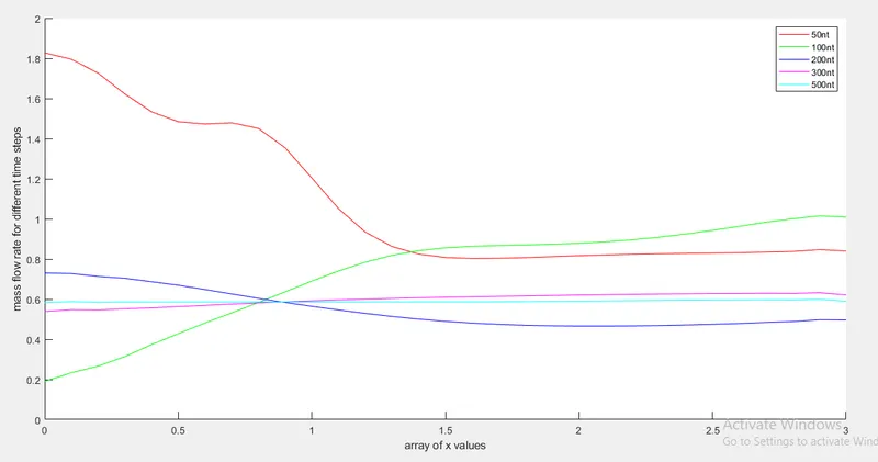
Plot of mass flow rate with varying time step:
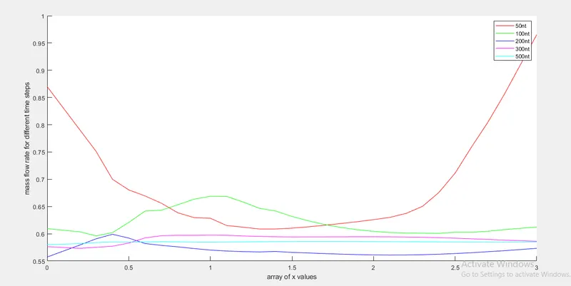
In the above plot we can find that the plot get stable at higher values of time step.
Matlab code for non-conservative form:
function [v_nc,T_nc,rho_nc,M_nc,m_nc,p_nc,v_th_nc,T_th_nc,rho_th_nc,M_th_nc,m_th_nc,p_th_nc] = nonconservative_solver(x,dx,nt,gamma,n,CFL,th)

%initial condition
rho_nc = 1 - 0.3416*x;
T_nc = 1 - 0.2314*x;
v_nc = (0.1+1.09*x).*T_nc.^(0.5);
A = 1+2.2*(x-1.5).^2;

for i=1:n
    dt_cal(i) = CFL*(dx/((T_nc(i).^(0.5))+(v_nc(i))));
end
dt = min(dt_cal);


nt = 1400;


for k = 1:nt

    rho_old = rho_nc;
    T_old = T_nc;
    v_old = v_nc;

    %predictor method

     for i=2:n-1
          %splitting equation for ease in understanding error
          dvdx = (v_nc(i+1) - v_nc(i))/dx;
          drhodx = (rho_nc(i+1) - rho_nc(i))/dx;
          dTdx = (T_nc(i+1) - T_nc(i))/dx ;
          dlogadx = (log(A(i+1)) - log(A(i)))/dx;

          %continuity equation
          %conservation of mass
          drhodt_p(i) = -rho_nc(i)*dvdx - rho_nc(i)*v_nc(i)*dlogadx - v_nc(i)*drhodx;

          %momentum equation
          dvdt_p(i) = -v_nc(i)*dvdx - ((1/gamma)*(dTdx+ (T_nc(i)/rho_nc(i))*drhodx));

          %energy equation
          dTdt_p(i) = -v_nc(i)*dTdx -((gamma-1)*T_nc(i)*(dvdx+ v_nc(i)*dlogadx));

          rho_nc(i) = rho_nc(i)+ drhodt_p(i)*dt;
          v_nc(i) = v_nc(i)+ dvdt_p(i)*dt;
          T_nc(i) = T_nc(i)+ dTdt_p(i)*dt;
     end

     %corrector step
     for i=2:n-1
          %splitting equation for ease in understanding error
          dvdx = (v_nc(i) - v_nc(i-1))/dx;
          drhodx = (rho_nc(i) - rho_nc(i-1))/dx;
          dTdx = (T_nc(i) - T_nc(i-1))/dx ;
          dlogadx = (log(A(i))- log(A(i-1)))/dx;

          %continuity equation
          %conservation of mass
          drhodt_c(i) = -rho_nc(i)*dvdx-rho_nc(i)*v_nc(i)*dlogadx-v_nc(i)*drhodx;

          %momentum equation
          dvdt_c(i) = -v_nc(i)*dvdx - ((1/gamma)*(dTdx+(T_nc(i)/rho_nc(i))*drhodx));

          %energy equation
          dTdt_c(i) = -v_nc(i)*dTdx - (gamma-1)*T_nc(i)*((dvdx)+(v_nc(i)*dlogadx));
end

 drhodt = 0.5*(drhodt_p + drhodt_c);
 dvdt = 0.5*(dvdt_p + dvdt_c);
 dTdt = 0.5*(dTdt_p + dTdt_c);

 for j=2:n-1
     rho_nc(j)= rho_old(j)+ drhodt(j)*dt;
     v_nc(j) = v_old(j) + dvdt(j)*dt;
     T_nc(j) = T_old(j) + dTdt(j)*dt;
 end

%boundry conditions
%inflow
v_nc(1) = 2*v_nc(2) - v_nc(3);

%outflow
v_nc(n) = 2*v_nc(n-1) - v_nc(n-2);
rho_nc(n) = 2*rho_nc(n-1) - rho_nc(n-2);
T_nc(n) = 2*T_nc(n-1) - T_nc(n-2);

M_nc = v_nc./(T_nc.^(0.5));
m_nc = v_nc.*A.*rho_nc;
p_nc = rho_nc.*T_nc;

v_th_nc(k) = v_nc(th);
T_th_nc(k) = T_nc(th);
M_th_nc(k) = M_nc(th);
p_th_nc(k) = p_nc(th);
rho_th_nc(k) = rho_nc(th);
m_th_nc(k) = m_nc(th);
%Plotting mass flow rate

figure(1)
hold on
if k==50
    plot(x,m_nc,'color','r')
elseif k==100
        plot(x,m_nc,'color','g')
elseif k==200
            plot(x,m_nc,'color','b')
elseif k==300
            plot(x,m_nc,'color','m')
elseif k==500
            plot(x,m_nc,'color','c')
            xlabel('array of x values')
            ylabel('mass flow rate for different time steps')
            legend('50nt','100nt','200nt','300nt','500nt')
end
end
hold on
figure(2)
subplot(2,2,1)
plot(x,rho_nc)
title('density vs length of nozzle')
xlabel('length of nozzle')
ylabel('density')

subplot(2,2,2)
plot(x,p_nc)
title('pressure vs length of nozzle')
xlabel('length of nozzle')
ylabel('pressure')

subplot(2,2,3)
plot(x,T_nc)
title('temperature vs length of nozzle')
xlabel('length of nozzle')
ylabel('temperature')

subplot(2,2,4)
plot(x,M_nc)
title('Mach number vs length of nozzle')
xlabel('length of nozzle')
ylabel('Mach number')

%variation of primitive variable with time step near a throat
hold on
figure(3)
subplot(2,2,1)
plot(linspace(1,nt,nt),rho_th_nc)
title('density at throat vs time step')
axis([0 1400 0.5 1.2])
xlabel('Time step')
ylabel('density at throat')

subplot(2,2,2)
plot(linspace(1,nt,nt),T_th_nc)
title('Temperature at throat vs time step')
axis([0 1400 0.7 1.1])
xlabel('Time step')
ylabel('Temperature at throat')

subplot(2,2,3)
plot(linspace(1,nt,nt),p_th_nc)
title('pressure at throat vs time step')
axis([0 1400 0.4 1.2])
xlabel('Time step')
ylabel('pressure at throat')

subplot(2,2,4)
plot(linspace(1,nt,nt),M_th_nc)
title('Mach number at throat vs time step')
axis([0 1400 0 2])
xlabel('Time step')
ylabel('Mach number at throat')
end
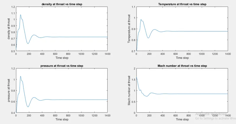
PLOTS:
Plot of primitive variables vs time step:
Plot for variation of primitive variables with the length of nozzle:
Plot of mass flow rate with varying time step:
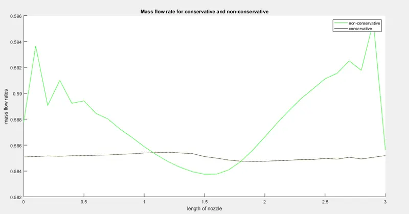
Comparison of mass flow rates for conservative and non-conservative form:
Time taken:
Time taken for non-conservative form = 5.77s
Time taken for conservative form = 33s
Variations with courant number:
As courant number increases we just see slight variations in the values of primitive variables and after it exceeds >1 the solution get blew up.
|
Courant number |
T/T0 |
M/M0 |
P/P0 |
ρ/ ρ0 |
|
0.5 |
0.841 |
0.978 |
0.548 |
0.652 |
|
0.7 |
0.849 |
0.926 |
0.568 |
0.670 |
|
0.9 |
0.848 |
0.924 |
0.568 |
0.669 |
|
1 |
0.848 |
0.922 |
0.568 |
0.669 |
|
1.1 |
0.848 |
0.921 |
0.567 |
0.669 |
|
1.2 |
0.848 |
0.920 |
0.567 |
0.669 |
|
1.3 |
Blew up |
Blew up |
Blew up |
Blew up |
|
Analytic solution |
0.833 |
1 |
0.528 |
0.634 |
Grid dependence:
|
Grid points |
T/T0 |
V/V0 |
P/P0 |
ρ/ ρ0 |
|
31 |
0.8410 |
0.896 |
0.5487 |
0.6524 |
|
61 |
0.8411 |
0.897 |
0.5486 |
0.6522 |
|
Analytic solution |
0.833 |
0.886 |
0.528 |
0.886 |
Initially we keep the grid points as 31 and calculate the value of primitive variables, Now as we increase the grid point to 61 we actually get a solution for primitive variable similar to previous condition, but it depends on the level of accuracy we need for a problem, and also the time for simulation decreases as we increase number of grids.
In this problem since by changing number of grid points does not effect the solution so its grid independent.
Conclusion:
The conservative form takes take more time then a non-conservative form but the accuracy of flux vectors used in conservative form is greater then primitive variables directly used in non-conservative form.
The value for mass flow rate of conservative form at throat have greater difference with analytic solution compared to non-conservative form.
Over all the non-conservative method is better compared to conservative method.
REFERANCES:
https://en.wikipedia.org/wiki/Isentropic_nozzle_flow
Basics of computational fluid dynamics- John D.Anderson, jr.